Unit 2.4: Systems and Classification of Systems#
This section is based on Section 1.5 of [Hsu, 2020].
Follow along at cpjobling.github.io/eg-150-textbook/signals_and_systems/systems

Subjects to be covered#
System Representation#
A system is a mathematical model of a physical process that relates the input (or excitation) signal to the output (or response) signal.
Let \(x\) and \(y\) be the input and output signals, respectively, of a system. Then the system is viewed as a transformation (or mapping) of \(x\) into \(y\). The transformation is represented by the mathematical notation
where \(\mathbf{T}\) is the operator representing some well defined rule by which \(x\) is transformed into \(y\).
The relationship is depicted graphically as shown in Fig. 25(a).
Multiple input and/or output systems are possible as shown in Fig. 25(b). In this module we will restrict our attention to the single-input, single-output case.
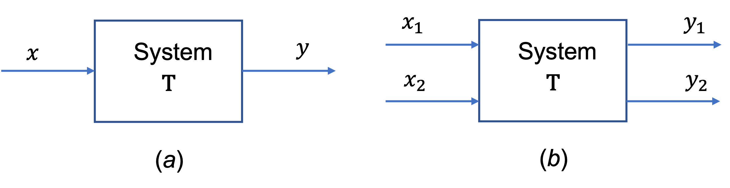
Fig. 25 System with single or multiple inputs and outputs#
Deterministic and Stochastic Systems#
If the input and output signals \(x\) and \(y\) are deterministic signals, then the system is called a deterministic system.
If the input and output signals \(x\) and \(y\) are random signals, then the system is called a stochastic system.
Continuous-Time and Discrete-Time Systems#
If the input and output signals 𝑥 and 𝑦 are continuous-time signals, then the system is called a continuous-time system (Fig. 26(a)).
If the input and output signals 𝑥 and 𝑦 are discrete-time signals or sequences, then the system is called a discrete-time system (Fig. 26(b)).
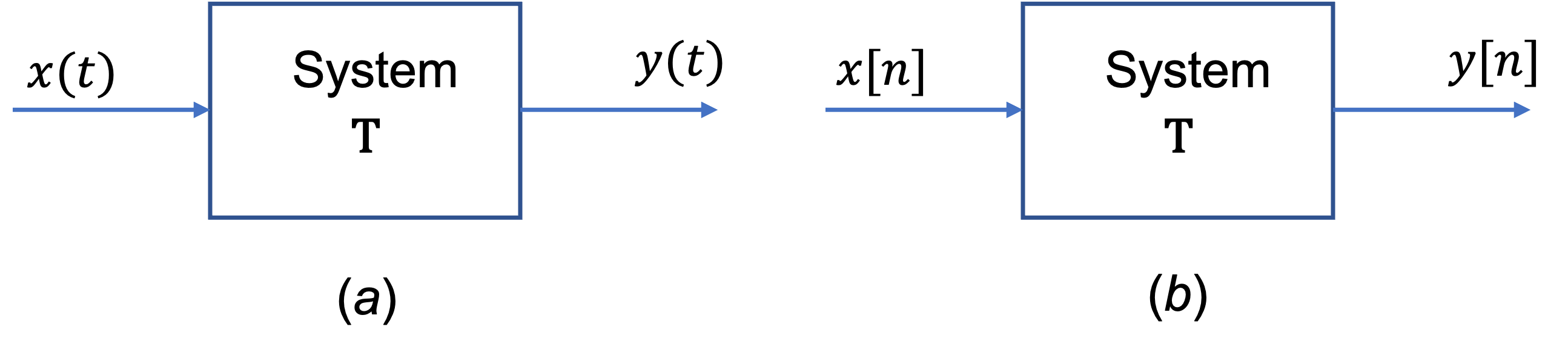
Fig. 26 (a) Continuous-time system; (b) discrete time system.#
Note that in a continuous-time system the input \(x(t)\) and \(y(t)\) are often expressed as a differential equation (see Exercises 4) and in a discrete-time system \(x[n]\) and \(y[n]\) are often expressed by a difference equation.
Systems with Memory and without Memory#
A system is said to be memoryless if the output at any time only depends on the input at the same time.
Otherwise the system is said to have memory.
A memoryless system#
An example of a memoryless system is a resistor \(R\) with and the input \(x(t)\) taken as the current and the voltage taken as the output \(y(t)\).

Fig. 27 A memoryless system: a resistor#
The input-output relationship (Ohm’s law) of a resistor is
A system with memory#
An example of a system with memory is a capacitor \(C\) with and the current as the input \(x(t)\) taken as the current and the voltage as the output \(y(t)\).
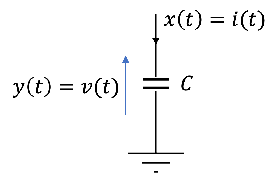
Fig. 28 A system with memory: a capacitor#
Then:
Causal and Non-Causal Systems#
A system is called causal if its output at the present time depends only on the present and/or past values of the input.
Thus, in a causal system, it is not possible to obtain an output before an input is applied to the system.
A system is called noncausal (or anticipative) if its output at the present time depends on future values of the input.
An example of a noncausal system is
Note that all memoryless systems are causal but not all vice versa.
Linear Systems and Nonlinear Systems#
If an operator \(\mathbf{T}\) satisfies the following two conditions, then \(\mathbf{T}\) is called a linear operator and the system represented by the linear operator \(\mathbf{T}\) is called a linear system:
Properties of Linear Systems#
1. Additivity#
Given that \(\mathbf{T}\left\{x_1\right\} = y_1\) and \(\mathbf{T}\left\{x_2\right\} = y_2\),
then
for any signals \(x_1\) and \(x_2\).
2. Homogeneity (or Scaling)#
for any signals \(x\) and any scalar \(\alpha\).
Nonlinear systems#
Any system that does not satisfy the additivity and homogeneity conditions is classified as a nonlinear system.
Superposition property#
The additivity and homogeneity conditions can combined in a single condition (known as the superposition property) as
where \(\alpha_1\) and \(\alpha_2\) are arbitrary scalars.
Example linear systems#
Examples of linear systems are the resistor and capacitor discussed earlier.
Example nonlinear systems#
Examples of nonlinear systems are
Zero input property#
Note that a consequence of the homegenity (or scaling) property of linear systems is that a zero input yields a zero output. This follows readily by setting \(\alpha = 0\) in the equation \(\mathbf{T}\left\{\alpha x\right\} = \alpha y\). This is another important property of linear systems.
Time-Invariant and Time-Varying Systems#
A system is called time-invariant if a time-shift (delay or advance) in the input signal causes the same time-shift in the output signal.
Thus for a continuous-time system, the system is time-invariant if
for any real value of \(\tau\).
Time-varying system#
A system that does not satisfy the equation \(\mathbf{T}\left\{x(t - \tau)\right\}=y(t - \tau)\) is called a time-varying system.
Testing for time-invariance#
To check for time invariance, we can compare the time-shifted output with the output produced by the time-shifted input (See Exercise 4.2: Capacitor circuit and Exercise 4.3: Signal modulator).
Linear Time-Invariant Systems#
If a system is linear and also time-invariant it is called a linear time-invariant (LTI) system.
All ths systems analysed in in the rest of the module and in EG-247 Digital Signal Processing and EG-243 Control Systems next year will be LTI systems.
Stable Systems#
A system is bounded-input/bounded-output (BIBO) stable if for any bounded input signal \(x\) defined by
the corresponding output \(y\) is also bounded defined by
where \(k_1\) and \(k_2\) are finite real constants.
Unstable systems#
An unstable system is one in which not all bounded inputs lead to a bounded output.
For example, consider the system where output
and input \(x(t)\) is the unit step \(u_0(t)\)
In this case \(x(t) = 1\) (so is bounded) but the output \(y(t)\) increases without bound as \(t\) increases.
Feedback Systems#
A special class of systems of great importance consists of systems having feedback.
In a feedback system, a portion of the output signal is fed back and added to the input as shown in Fig. 29.

Fig. 29 A feedback system with negative feedback: \(e(t) = x(t) - y(t)\).#
You will see examples of systems with feedback when you study op-amp circuits in EG-152 Practical Electronics, the simple closed-loop systems to be studied in EG-142 Instrumentation and Control. Feedback, and its impact on system stability, is also the basis of control theory to be studied next year in EG-243 Control Systems.
Exercises 4#
Exercise 4.1: RC Circuit#
MATLAB Example
We will solve this example by hand and then give the solution in the MATLAB lab.

Fig. 30 RC circuit#
Consider the RC circuit shown in Fig. 30. Find the relationship between the input \(x(t)\) and the output \(y(t)\)
(a) If \(x(t) = v_s(t)\) and \(y(t) = v_c(t)\).
(b) If \(x(t) = v_s(t)\) and \(y(t) = i(t)\).
For the answer, refer to the lecture recording or see solved problem 1.32 in [Hsu, 2020].
Exercise 4.2: Capacitor circuit#
MATLAB Example
We will solve this example by hand and then give the solution in the MATLAB lab.
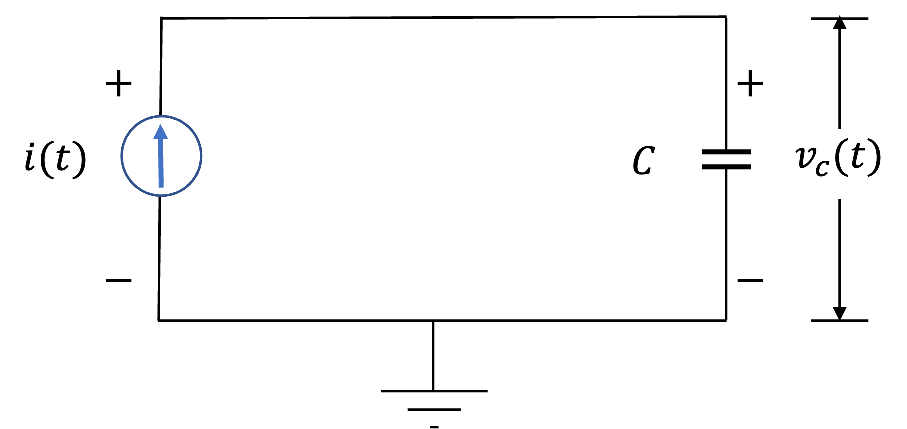
Fig. 31 A capacitor circuit.#
Consider the capacitor shown in Fig. 31. Let the input \(x(t) = i(t)\) and the output \(y(t) = v_c(t)\).
(a) Find the input-output relationship.
(b) Determine whether the system is (i) memoryless, (ii) causal, (iii) linear, (iv) time invariant, or (v) stable.
For the answer, refer to the lecture recording or see solved problem 1.33 in [Hsu, 2020].
Exercise 4.3: Signal modulator#
MATLAB Example
We will solve this example by hand and then give the solution in the MATLAB lab.
Consider the system shown in Fig. 32. Determine whether it is (a) memoryless, (b) causal, (c) linear, (d) time invariant, or (e) stable.
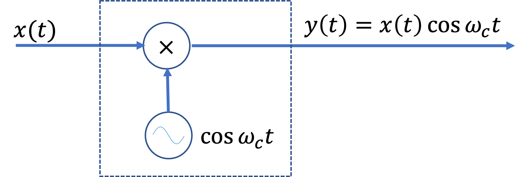
Fig. 32 A signal modulator#
For the answer, refer to the lecture recording or see solved problem 1.34 in [Hsu, 2020].
Exercise 4.4#
A system has the input-output relationship given by
Show that this system is nonlinear.
For the answer, see the solved problem 1.35 in [Hsu, 2020].
Exercise 4.5#
Consider the system whose input-output relationship is given by the linear equation
where \(x\) and \(y\) are the input and output respectively and \(s\) and \(b\) are constant. Is this system linear?
For the answer, see the solved problem 1.40 in [Hsu, 2020].
Exercise 4.6#
(a) Show that the causality for a continuous-time linear system is equivalent to the following statement: For any time \(t_0\) and any input \(x(t)\) with \(x(t) = 0\) for \(t \le t_0\), the output \(y(t)\) is zero for \(t \le t_0\).
(b) Find a nonlinear system that is causal but does not satisfy this condition.
(c) Find a nonlinear system that satisfies this condition but is not causal.
For the answer, see the solved problem 1.43 in [Hsu, 2020].
Exercise 4.7#
Let \(\mathbf{T}\) represent a continuous-time LTI system. Then show that
where \(s\) is a complex variable and \(\lambda\) is a complex constant.
Note
The solution to this problem is part of a journey that leads us from continuous-time LTI systems to the Laplace transform. I have therefore included the solution in full.
Solution#
Let \(y(t)\) be the output of the system with input \(x(t)=e^{st}\). Then
Since the system is time-invariant, we have
for arbitrary real \(t_0\).
Since the system is linear, we have
Hence,
Setting \(t=0\), we obtain
Since \(t_0\) is arbitrary, by changing \(t_0\) to \(t\), we can rewrite \(y(t_0) = y(0)e^{st_0}\) as
or
where \(\lambda = y(0)\).
Important
Note
In mathematical language, a function \(x(\cdot)\) satisfying the equation
is called an eigenfunction (or characteristic function) corresponding to the eigenvalue \(x(\cdot)\).
Thus, the solution to the previous example indicates that the complex exponential function is an eigenfunction of an LTI system.
Unit 2.4 Takeaways
In this lecture we have started our look at systems and the classification of systems.
In particular we have looked at
A continuous-time system is linear if superposition holds. That is
where \(\alpha_1\) and \(\alpha_2\) are arbitrary scalars.
A continuous-time system is time-invariant if
for any real value of \(\tau\).
For continuous-time LTI system represented by \(\mathbf{T}\)
where \(s\) is a complex variable and \(\lambda\) is a complex constant. In this formulation \(e^{st}\) is called an eigenfunction of \(\mathbf{T}\) and \(\lambda\) is the eigenvalue. See Eigenfunctions of Continuous-Time LTI Systems for the further development of this idea.
A system is bounded-input/bounded-output (BIBO) stable if for any bounded input signal \(x\) defined by
the corresponding output \(y\) is also bounded defined by
where \(k_1\) and \(k_2\) are finite real constants.