Unit 5.2: More on the Qualitative and Quantitative Response of First- and Second-Order Poles

Unit 5.2: More on the Qualitative and Quantitative Response of First- and Second-Order Poles#

Follow along at cpjobling.github.io/eg-150-textbook/poles_and_zeros/second_order_properties

QR Code for this lecture

Acknowledgements#

The notes for this unit have been influenced by the MATLAB LiveScript PoleZeroAnalysis.mlx from the MathWorks curriculum module Transfer Function Analysis of Dynamic Systems [Allie, 2024]. You will find some useful interactive applications with which you can explore the concepts presented here. Some of these will be deomostrated in the lecture.

The examples have been inspired by the recording of the second half of the video recording of Stephen Boyd’s 1999 lecture 10 (delivered at Stanford University) which itself is based on Qualitative properties of signals & Laplace transforms [Boyd, 1993].

You can watch the video on YouTube here:

Agenda#

Quantitative behaviour of real poles
Natural frequency
Step-response of a second-order system
Useful quantifiers that result from step response
Exercises 16

Quantitative behaviour of real poles#

In Qualitative properties of terms we stated that a response term that corresponds to a real pole $s = σ$ will result in a growing expontial if $σ > 0$ and a decaying exponential if $σ < 0$ .

We didn’t quantify these effects, so it is useful to do so here.

Rate of exponential growth#

Given that the rational polynomial $F (s)$ representing the Laplace transfer of a signal or system has a pole $s = σ$ , one of the terms in the partial fraction expansion will be

\frac{r_{σ}}{s - σ}

where $r_{σ}$ is the residue of the pole.

The corresponding term in $f (t)$ will be $r_{σ} e^{σ t}$ .

This will be a growing exponential for which the doubling time is a useful measure of the growth rate.

Given that at time $t = 0$ , $r_{σ} e^{0} = r_{σ}$ , the doubling time $T$ is the time for which:

\begin{array}{r} \begin{aligned} r_{σ} e^{σ T} & = 2 r_{σ} \\ e^{σ T} & = 2 \\ σ T & = \log_{e} 2 \\ T & = \frac{\log_{e} 2}{σ} = \frac{0.693147180559945}{σ} \approx \frac{0.7}{σ} . \end{aligned} \end{array}

Example 7#

Plot the response of the pole

\frac{10}{s - 0.1}

and confirm that the doubling time is around 7 seconds.

Solution to example 7#

Done in MATLAB

format compact
clear variables

sigma = 0.1;
% Doubling time
T = log(2)/sigma

T = 6.9315

% Plot
t = linspace(0,15,100);
plot(t,10*exp(sigma*t)),ylim([0,50]),grid

% Plot and label lines: first doubling
line([T,T],[0,20],'Color','r','LineStyle','--')
line([0,T],[20,20],'Color','r','LineStyle','--')
hold on
plot(T,20,'o')
text(3,22,'First doubling')
% Plot and label lines: second doubling
plot(2*T,40,'o')
line([2*T,2*T],[0,40],'Color','g','LineStyle','--')
line([0,2*T],[40,40],'Color','g','LineStyle','--')
text(10,42,'Second doubling')
% Label graph
title('Exponential growth'),
ylabel('f(t) = 10*exp(0.1*t)'),xlabel('Time t [s]')
hold off

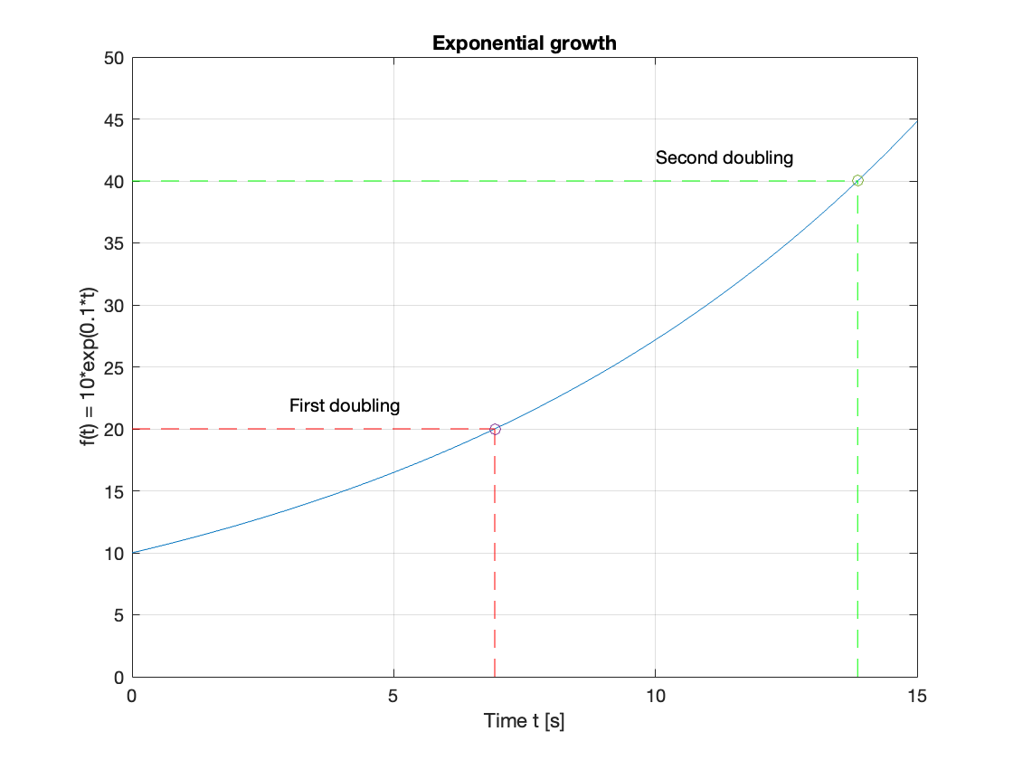
../_images/2002a560448c8b92003989bfef3a43a47a0c02ed487dbb38bfd8310cc2f2105a.png

Given that $σ = 0.1$ , the doubling time $T \approx 0.7 / σ = 7$ s. The initial value is $10$ at $t = 0$ s. It has doubled to $20$ at $t \approx 7$ s, and has doubled again to $40$ at $t \approx 14$ .

We have added the exact solutions to the plot.

The MATLAB code to reproduce this result is given in example7.mlx

Rate of exponential decay#

If $F (s)$ has a pole $s = - σ$ , one of the terms in the partial fraction expansion will be

\frac{r_{σ}}{s + σ}

where $r_{σ}$ is the residue of the pole.

The corresponding term in $f (t)$ will be $r_{σ} e^{- σ t}$ .

This will be a decaying exponential for which the time constant $τ = 1 / | σ |$ is a useful measure of the decay rate.

Putting the time constant into the response equation

r_{σ} e^{- σ τ} = r_{σ} e^{- 1} = 0.367879441171442 r_{σ} \approx 0.37 r_{σ} .

Thus the response reaches around $37 %$ of its initial value in $τ = 1 / | σ |$ s.

Another measure of decay that is sometimes used is the value of $t$ for which the response reaches $1 %$ of its initial value.

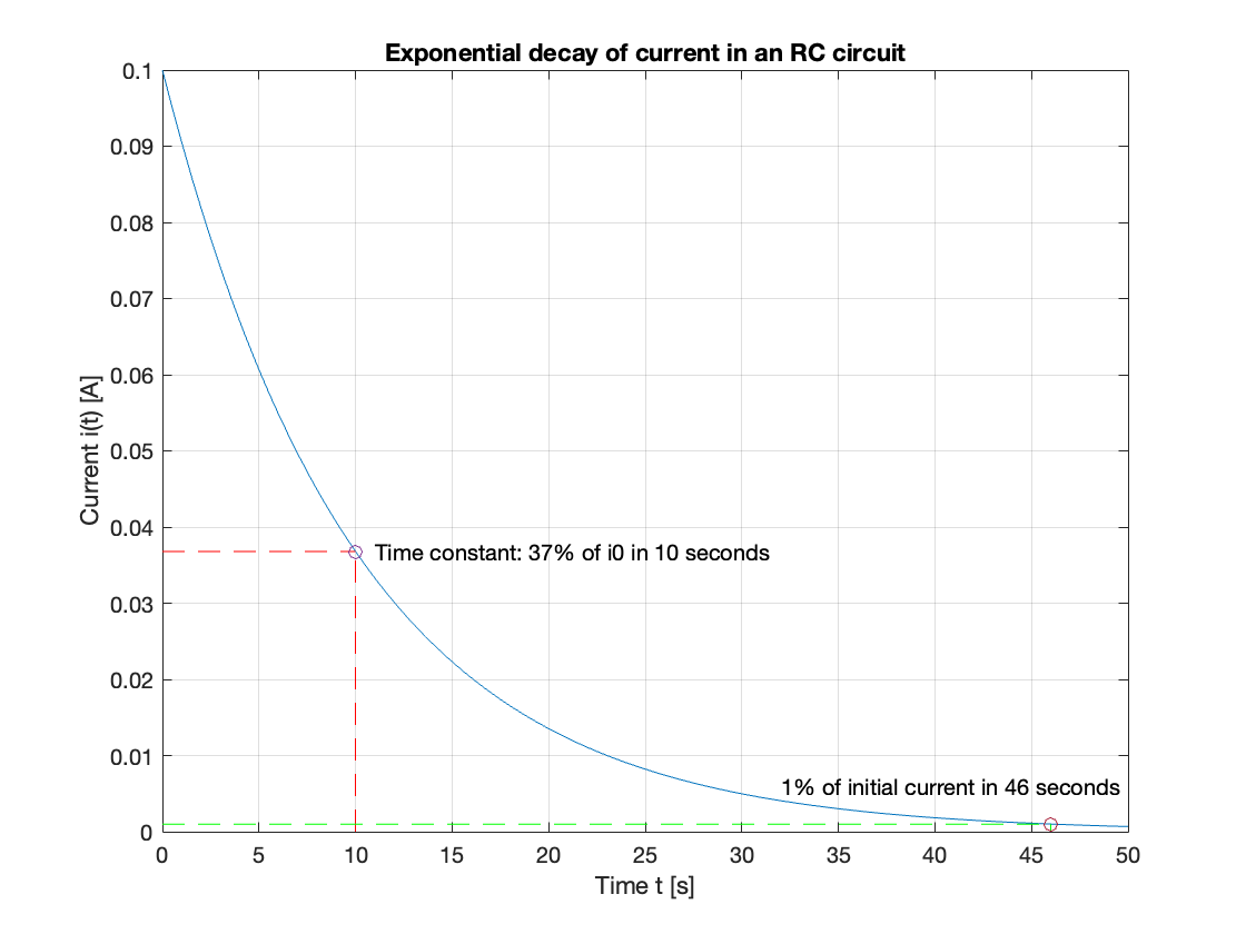
\begin{array}{r} \begin{aligned} 0.01 r_{σ} & = r_{σ} e^{- t / τ} \\ 0.01 & = e^{- t / τ} \\ \log_{e} (0.01) & = - t / τ \\ t_{1 %} & \approx 4.6 τ \end{aligned} \end{array}

Example 8#

The current in the RC circuit shown in Fig. 41 has the transform

I (s) = \frac{1 / R C}{s + 1 / R C}

If $R = 1$ M $Ω$ and $C = 10$ $μ$ F, determine:

(a) The initial current $i (0)$ .

(b) The time constant $τ$ .

(c) The time at which the current decays to 1% of $i (0)$ .

Solution to example 8#

(a) The initial current is given by[1]

lim_{s \to \infty} s I (s) = lim_{s \to \infty} s \frac{1 / R C}{s + 1 / R C} = 1 / R C .

Given the component values of $R$ and $C$ , $i (0) = 1 / R C = 100$ mA.

(b) The time constant $τ = R C = 10$ s.

(c) The time at which the current decays to 1% of $i (0)$ is 46 s.

MATLAB confirmation

t = linspace(0,50,100);
R = 1e6; C = 10e-6;
sigma = -1/(R*C);
% Time constant and initial current
tau = 1/abs(sigma); i0 = 1/(R*C);
% Plot
plot(t,i0*exp(sigma*t)),grid
% Plot and label lines: time constant
line([tau,tau],[0,i0*exp(-1)],'Color','r','LineStyle','--')
line([0,tau],[i0*exp(-1),i0*exp(-1)],'Color','r','LineStyle','--')
text(tau+1,i0*exp(-1),'Time constant: 37% of i0 in 10 seconds')
hold on
plot(tau,i0*exp(-1),'o')
% Plot and label lines: 1% point
line([4.6*tau,4.6*tau],[0,0.01*i0],'Color','g','LineStyle','--')
line([0,4.6*tau],[0.01*i0,0.01*i0],'Color','g','LineStyle','--')
plot(4.6*tau,0.01*i0,'o')
text(32,0.01*i0+0.005,'1% of initial current in 46 seconds')
% Label graph
title('Exponential decay of current in an RC circuit'),
ylabel('Current i(t) [A]'),xlabel('Time t [s]')
hold off

../_images/6ee5b0ca8def1168b1a32d57f724055b6d7592e4051d1b7693ddbc0caca1978b.png

The MATLAB code to reproduce this result is given in example8.mlx

Natural frequency#

The locations of the poles in the $s$ -plane determine the natural oscillation frequencies present in the system.

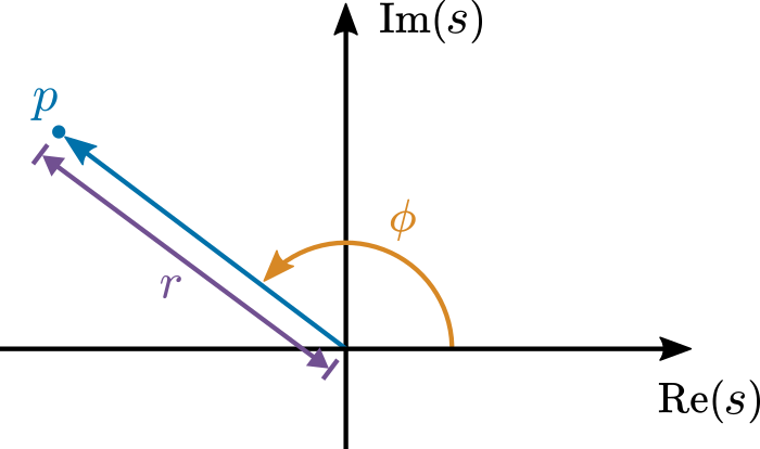
Consider a pole in the complex plane illustrated in Fig. 78

Phase phi and magnitude r of pole p shown in the complex plane — Fig. 78 Phase $ϕ$ and magnitude $r$ of pole $p$ shown in the complex plane#

The natural (undamped) frequency (in rad/s) contributed by a pole $p$ is the pole magnitude, $r = | p |$ .
The phase, $ϕ = \arg p$ , determines the relative strength of the oscillatory component.

Analysis of a second-order system#

Second-order systems with a pair of conjugate poles and no zeros are useful for illustrating the natural frequency response analytically. It is helpful to write this type of system in the form:

G (s) = \frac{K}{s^{2} + 2 ζ ω_{n} s + ω_{n}^{2}}

where

$K$ is the gain coefficient
$ζ$ is the damping ratio already introduced in Complex poles: Damping ratio \zeta and quality factor Q
and $ω_{n}$ is the (undamped) natural frequency.

These parameters are helpful for drawing a connection between the natural response of the system and the properties of the poles. In this section, the poles of the second-order system will be analytically computed and related to the natural response of the system.

Pole analysis#

The poles of the system occur when the denominator is zero:

p_{1, 2} = - ζ ω_{n} \pm ω_{n} \sqrt{ζ^{2} - 1}

For simplicity, consider $ζ \in [0, 1)$ . In this case, the poles are

p_{1, 2} = - ζ ω_{n} \pm j ω_{n} \sqrt{1 - ζ^{2}}

As stated above, the natural frequency is defined as the magnitude of the pole. The magnitude is computed as :

\sqrt{{Re}^{2} + {Im}^{2}}

Using the definitions illustrated in Fig. 76, $Re = - σ = - ζ ω_{n}$ and $Im = ω = ω_{n} \sqrt{1 - ζ^{2}}$ , so :

\begin{array}{r} \begin{aligned} | p | & = \sqrt{σ^{2} + ω^{2}} \\ = \sqrt{(- ζ ω_{n})^{2} + (\pm ω_{n} \sqrt{1 - ζ^{2}})^{2}} \\ = \sqrt{ζ^{2} ω_{n}^{2} + ω_{n}^{2} (1 - ζ^{2})} \\ = | ω_{n} | \end{aligned} \end{array}

This illustrates why this form of the equation is used: the natural frequency is the parameter $ω_{n}$ .

The damping ratio $ζ$ determines the relative strength of the exponential part of the response.

As $ζ \to 1$ , the complex part of the pole tends to zero, implying less oscillatory and stronger exponential behavior.

For stable systems, that implies greater damping.

The gain coefficient $K$ affects the magnitude of the response, not the time-dependent behavior.

Natural response#

The impulse response of a system $H (s)$ is also called the natural response. The natural response $y (t)$ is computed by taking the inverse Laplace transform of

\frac{Y (s)}{X (s)} = \frac{Y (s)}{1} = \frac{K}{s^{2} + 2 ζ ω_{n} s + ω_{n}^{2}}

because the impulse $x (t) = δ (t)$ has a Laplace transform $1$ . You can find the response’s analytic form by referring to a table or using the MATLAB ilaplace function.

syms s t zeta omega_n K Y(s) y(t)
assume(t > 0)
Y(s) = K/(s^2 + 2*zeta*omega_n*s + omega_n^2)

Y (s) = \frac{K}{{ω_{n}}^{2} + 2 ζ ω_{n} s + s^{2}}

y(t) = ilaplace(Y) % The impulse response in the time domain

y (t) = \frac{K e^{- ω_{n} t ζ} \sin (ω_{n} t \sqrt{1 - ζ^{2}})}{ω_{n} \sqrt{1 - ζ^{2}}}

Gives the result

(60)#

y (t) = \frac{K e^{- ζ ω_{n} t} \sin (ω_{n} t \sqrt{1 - ζ^{2}})}{ω_{n} \sqrt{1 - ζ^{2}}}

Notice that the impulse response is a product of an exponential and sine function. From these functions observe that:

The sine function frequency (in rads/s) is $ω_{n} \sqrt{1 - ζ^{2}}$ . If the damping $ζ = 0$ , then the frequency is $ω_{n}$ . This is the reason $ω_{n}$ is often referred to as the undamped natural frequency.
The rate of decay of the exponential damping function is $ζ ω_{n}$ .
The gain parameter $K$ only contributes as a constant multiplier to the magnitude of the response.

Step-response of a second-order system#

The step response of a system $H (s)$ is often computed. The step response $y_{s} (t)$ is determined by taking the inverse Laplace transform of

Y (s) = \frac{1}{s} (\frac{ω_{n}^{2}}{s^{2} + 2 ζ ω_{n} s + ω_{n}^{2}})

because the step function $x (t) = u_{0} (t)$ has a Laplace transform $1 / s$ . You can find the response’s analytic form by taking partial fraction expansion of $Y (s)$ and then referring to a table of Laplace transforms.

Here we will state, without proof, that the step response will be

(61)#

y_{s} (t) = (1 - e^{- σ t} (\cos (ω t) + \frac{σ}{ω} \sin (ω t))) u_{o} (t)

where :

$ω = ω_{n} \sqrt{1 - ζ^{2}}$ is the imaginary part of the system’s complex pole pair, sometimes called the damped natural frequency
$σ = ζ ω_{n}$ is the magnitide of the real part of the system’s complex pole pair
$ϕ = \tan^{- 1} ζ / (1 - ζ^{2})$ is the phase shift.

Note

The proof requires us to complete the square in the denominator of the term with the complex roots

(s^{2} + 2 ζ ω_{n} + ω_{n}^{2}) = {(s + ζ ω_{n})}^{2} + (ω_{n}^{2} (1 - ζ^{2}))

Then take the PFE of the terms assuming that the complex poles will yield terms:

(62)#

r_{1} \frac{s + ζ ω_{n}}{{(s + ζ ω_{n})}^{2} + {(ω_{n} \sqrt{1 - ζ^{2}})}^{2}} + r_{2} \frac{ω_{n} \sqrt{1 - ζ^{2}}}{{(s + ζ ω_{n})}^{2} + {(ω_{n} \sqrt{1 - ζ^{2}})}^{2}}

Making the substitutions $σ = ζ ω_{n}$ and $ω = ω_{n} \sqrt{1 - ζ^{2}}$ we can simplify (62) to

(63)#

r_{1} \frac{s + σ}{{(s + σ)}^{2} + ω^{2}} + r_{2} \frac{ω}{{(s + σ)}^{2} + ω^{2}}

The step-response terms will then be

r_{1} e^{- σ t} \sin (ω t) + r_{2} e^{- σ t} \cos (ω t)

Having computed the residues $r_{1}$ and $r_{2}$ the sine and cosine terms can be combined to give the final $e^{- σ t} \cos (ω t + ϕ)$ expression.

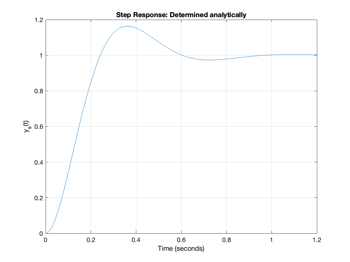
Example 9#

Determine the step response for a second order system with $ω_{n} = 10$ rad/s and $ζ = 0.5$ . Confirm your result using (61) and the tf and step functions.

Solution to example 9#

Analytical solution using the symbolic math toolbox

syms Y_s(s) y_s(t)
zeta = 0.5; omega_n = 10;
X(s) = 1/s;
H(s) = omega_n^2/(s^2 + 2*zeta*omega_n*s + omega_n^2);
Y_s(s) = H(s)*X(s)

Y_{s} (s) = \frac{100}{s (s^{2} + 10 s + 100)}

(64)#

Y_{s} (s) = \frac{100}{s (s^{2} + 10 s + 100)}

% step response
y_s(t) = ilaplace(Y_s(s))

y_{s} (t) = 1 - e^{- 5 t} (\cos (5 \sqrt{3} t) + \frac{\sqrt{3} \sin (5 \sqrt{3} t)}{3})

Gives the result

(65)#

y_{s} (t) = 1 - e^{- 5 t} (\cos (5 \sqrt{3} t) + \frac{\sqrt{3} \sin (5 \sqrt{3} t)}{3})

Plot the solution

fplot(y_s(t)*heaviside(t),[0,1.2]),ylim([0,1.2]),grid
xlabel('Time (seconds)'),ylabel('y_s(t)'),...
title('Step Response: Determined analytically')

../_images/34d0bcf3c2cd33ba5b13fdfe735a021ed006d16fd3a25fd947785c9486d4fba7.png

Confirming the result with (61) we get:

sigma = zeta*omega_n;
omega = omega_n*sqrt(1 - zeta^2);
% Compute response using the formula
t = linspace(0,1.2,100);
yst = (1 - exp(-sigma*t).*(cos(omega*t)+(sigma/omega)*sin(omega*t)));

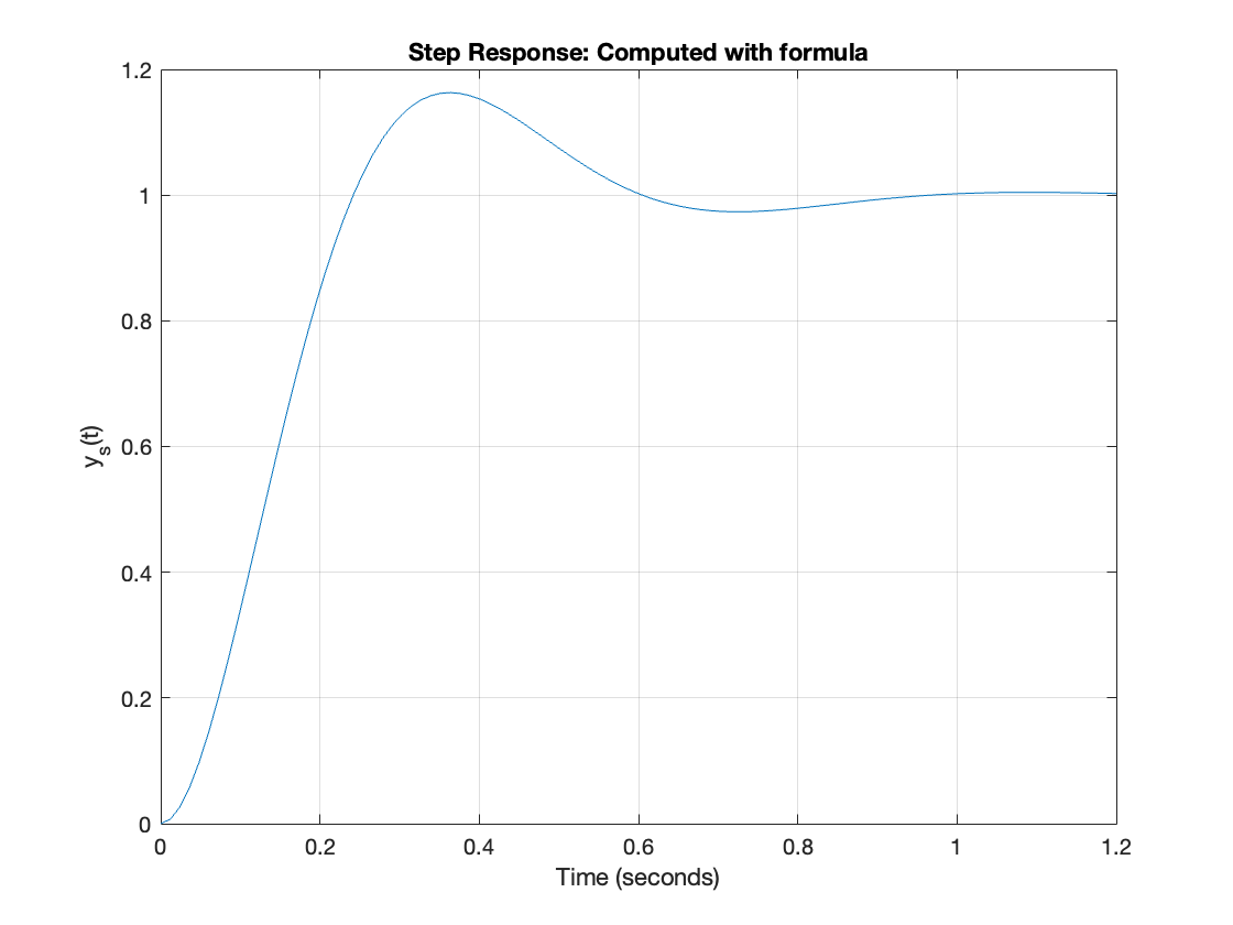
Plot the result

plot(t,yst),grid,...
xlabel('Time (seconds)'),ylabel('y_s(t)'),...
title('Step Response: Computed with formula')

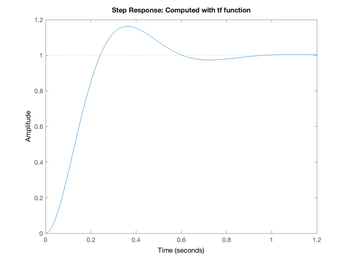
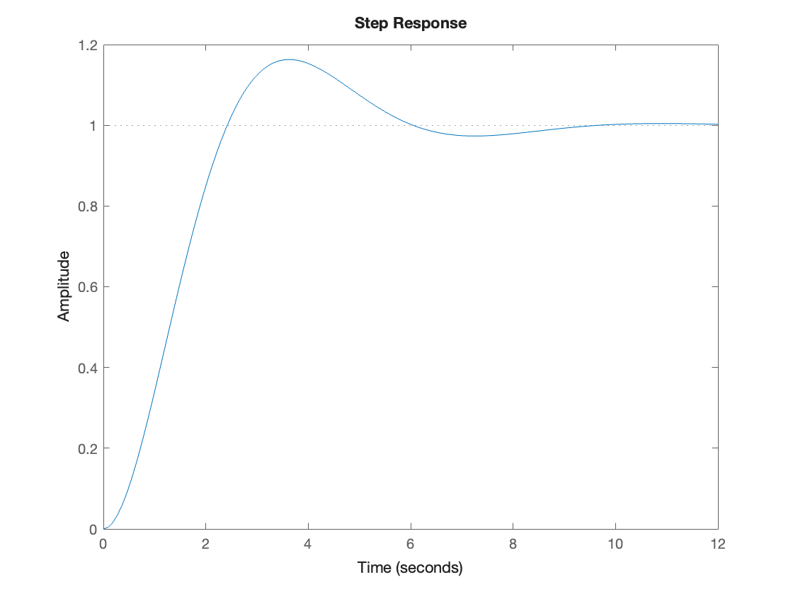
../_images/04ae2173e52357d8fbe6214baf743eb2ec72c47b589212b6309386368b34f349.png

Using the tf and step functions we get:

num = omega_n^2; den = [1 2*zeta*omega_n,omega_n^2];
Hs = tf(num,den)

Hs

  ----------------

  s^2 + 10 s + 100

Continuous-time transfer function.

step(Hs),title('Step Response: Computed with tf function')

../_images/246077ea6c1a97d17a4a6da4ba0ce2341038d3cf6cc191c7e6da650313fc78a5.png

The MATLAB code to reproduce this result is given in example9.mlx

Useful quantifiers that result from step response#

The relationship between the pole locations and the step response are summarized in Fig. 79 [2]

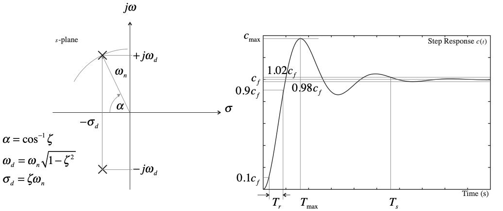
Fig. 79 Relationship between poles and step response#

Knowledge of the location of the poles and their damping ratio and natural frequency are useful for qualtitaive anaysis of the response of a complex pole pair. There are also a number of parameters that quantively define the features of the step response which we may be interested in. These are shown in the right-hand picture of Fig. 80. Knowledge of the poles allows us to predict the step response. But also, usefully for many design problems, knowledge of the step response allows us to predict the location of the poles.

We will explore these ideas in the following sections.

Poles#

The location of the system poles is important and can be obtained by factorizing the denominator of $H (s)$ either symbolically or numerically. There is also a handy function pole which will take these values from a transfer function.

We will illustrate these with the example used in Example 9.

First we set up the system function $H (s)$

syms s t
zeta = 0.5; omega_n = 10;
H = omega_n^2/(s^2 + 2*zeta*omega_n*s + omega_n^2)

H = \frac{100}{s^{2} + 10 s + 100}

Find the poles symbolically

[num,den] = numden(H);
symbolicPoles = factor(den,'FactorMode','full') % FactorMode needed to reduce quadratic

s y m b o l i c P o l e s = (\begin{array}{cc} s + 5 + 5 \sqrt{3} i & s + 5 - 5 \sqrt{3} i \end{array})

Factors interpreted as

(s + 5 + j 5 \sqrt{3}) (s + 5 - j 5 \sqrt{3})

Now find the poles numerically

% Convert symbolic polynomials to numeric polynomials
n = sym2poly(num); d = sym2poly(den);

% Compute the roots
den_poles = roots(d)

den_poles = 
  -5.0000 + 8.6603i
  -5.0000 - 8.6603i

FInally, from the transfer function model

Hs = tf(n,d);

poles = pole(Hs)

poles = 
  -5.0000 + 8.6603i
  -5.0000 - 8.6603i

Damping ratio and natural frequencies#

These are most conveniently obtained from the transfer function using the damp function.

[wn,z] = damp(Hs)

wn = 2×1 double
   10.0000
   10.0000

z = 2×1 double
    0.5000
    0.5000

The function damp can also return the poles

[wn,z,p] = damp(Hs)

wn = 2×1 double
   10.0000
   10.0000

z = 2×1 double
    0.5000
    0.5000

p = 
  -5.0000 + 8.6603i
  -5.0000 - 8.6603i

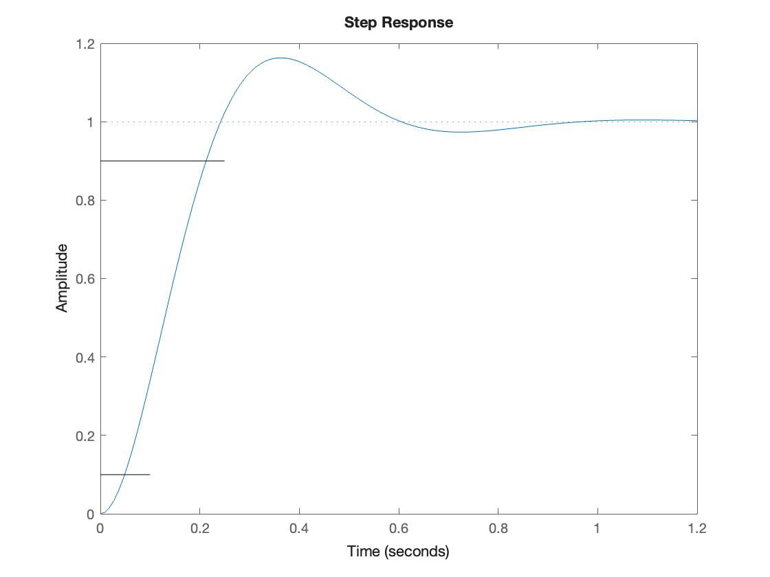
Rise-time#

The rise time $T_{r}$ is a measure of the speed of response of a system. It is usually taken to be the time taken to transition from 10% to 90% of the final value in the initial rise of the response. It is shown in Fig. 80.

The rise-time depends on $ω_{n}$ but its actual value is also dependent on the damping ratio $ζ$ so we rely on a calibration curve such as that shown in Fig. 80.

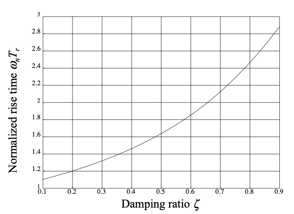
Fig. 80 Damping ratio as a function of normalised rise-time for a second-order underdamped response#

For the problem being considered $ζ = 0.5$ , so $ω_{n} T_{r} \approx 1.65$ giving

T_{r} \approx \frac{1.65}{ω_{n}} = \frac{1.65}{10} = 0.165 s .

step(Hs),line([0,0.1],[0.1,0.1]),line([0,0.25],[0.9,0.9])

../_images/4cee22c7123b7767395bb1a79c772ffba79315e53b7257e811fddc5acb0590dd.png

Settling time#

The settling time $T_{s}$ is defined as the time taken for the peaks of the oscillations in the step response to be bounded by some arbitrary limit. In Fig. 80 the bounds have been set to 2%.

The actual setting time is related to the real part of the poles and, for this case,

2 % T_{s} \approx \frac{4}{ζ ω_{n}}

For our example

Ts = 4/(zeta*omega_n) % seconds

Ts = 0.8000

step(Hs),line([0,1.2],[1.02,1.02]),line([0,1.2],[0.98,0.98])

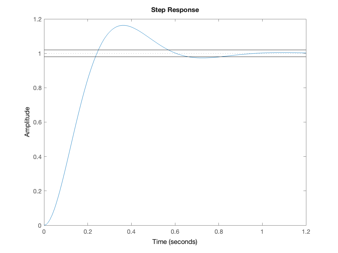
../_images/9e7e581815f81abe19389f5486ea856433b56f3db163078858a17daabafb26de.png

The value looks about right!

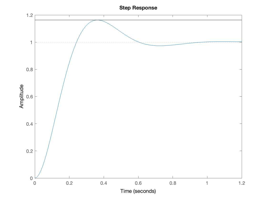
Peak overshoot#

The peak overshoot is a measure of damping in a system and is the height of the first peak ( $C_{max}$ in Fig. 80). It is usually quoted as a percentage of the final value.

% OS = \exp (\frac{- ζ π}{\sqrt{1 - ζ^{2}}}) \times 100

If we know the peak overshoot, we can calculate the damping ratio $ζ$ using the formula:

ζ = \frac{- \log_{e} (% OS / 100)}{\sqrt{π^{2} + \log_{e}^{2} (% OS / 100)}}

For our example

POS = exp(-zeta*pi/sqrt(1 - zeta^2))*100 % OS

POS = 16.3034

OS = 1 + POS/100; % OS 
step(Hs),line([0,1.2],[OS,OS])

../_images/e516a3d367f7dfe84d38034879be75a6c95c02561a935b8093cc24354411198c.png

Reverse formula check

z = -log(POS/100)/sqrt(pi^2 + log(POS/100)^2)

z = 0.5000

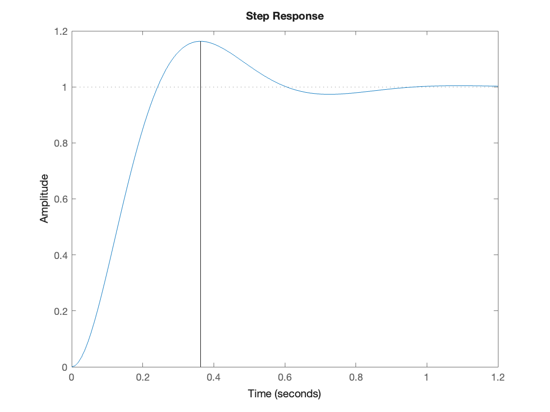
Peak time#

We sometimes compute the peak time $T_{p}$ , which is the time at which the first peak occurs. It depends on the damped natural frequency:

T_{p} = \frac{π}{ω_{d}} = \frac{π}{ω_{n} \sqrt{1 - ζ^{2}}}

For our example

Tp = pi/(omega_n*sqrt(1 - zeta^2))

Tp = 0.3628

step(Hs),line([Tp,Tp],[0,1.16304])

../_images/28f17bde19aaff45afad32696d7304f1e8dacbbaf9075e5b87fa373df0b6681c.png

List all properties#

MATLAB provides a useful function stepinfo that computes a step response for a system and takes measurements of the response to summarize the useful quantitative data defined above as well as a few more quantities.

stepinfo(Hs)

ans = struct with fields:
         RiseTime: 0.1639
    TransientTime: 0.8076
     SettlingTime: 0.8076
      SettlingMin: 0.9315
      SettlingMax: 1.1629
        Overshoot: 16.2929
       Undershoot: 0
             Peak: 1.1629
         PeakTime: 0.3592

You should compare the values computed with the approximations given in this section.

Exercises 16#

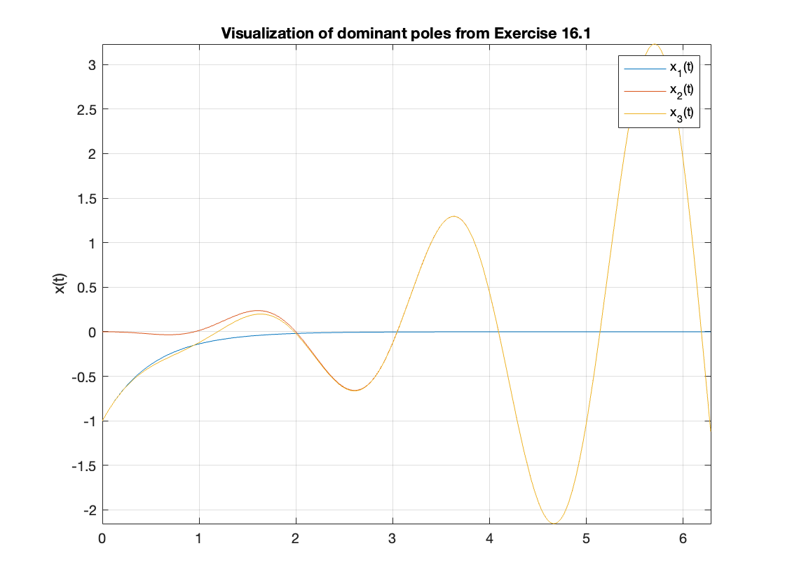
Exercise 16.1: Qualitative analysis#

A signal or system response $f (t)$ contains the terms

(66)#

\dots - e^{- 2 t} - 0.1 t^{2} \cos (3 t + 5) \dots

(a) How many poles are there in $F (s)$ ?

(b) What is the nature of the response due to the terms given in (66)?

(c) Which are the dominant poles?

MATLAB visualization

syms t
x_1 = -exp(-2*t)
x_2 = -0.1*t^2*cos(3*t + 5)
x_3 = x_1 + x_2
T = 2*pi/3; % Period of sinusoidal term
fplot(x_1,[0,3*T])
hold on
fplot(x_2,[0,3*T])
fplot(x_3,[0,3*T])
grid, title('Visualization of dominant poles from Exercise 16.1'),ylabel('x(t)')
legend('x_1(t)','x_2(t)','x_3(t)')
hold off

x_{1} = - e^{- 2 t}

x_{2} = - \frac{t^{2} \cos (3 t + 5)}{10}

x_{3} = - e^{- 2 t} - \frac{t^{2} \cos (3 t + 5)}{10}

../_images/052bea78fd0ae1af5c9cccaaf480dd1b5e235e33383fc61b441b57a5d65fdd8f.png

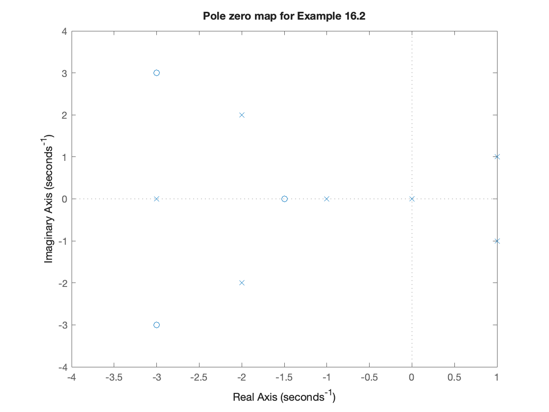
Exercise 16.2: Qualitative and quantitative analysis#

A system has poles $s = 0, 1 \pm j, - 1, - 2 \pm j 2, - 3$ and zeros at $s = - 1.5, - 3 \pm j 3$ .

(a) Give the transfer function $F (s) = b (s) / a (a)$

(b) Plot the poles on a pole zero map

(c) Give the time constant $τ$ , doubling time $T$ , damping ratio $ζ$ , angle $θ$ , natural frequency $ω_{n}$ , and quality factor $Q$ as appropriate for each pole or pole pair.

(d) How do the zeros affect the response $f (t)$ ?

(e) Which is the dominant pole?

(f) Will the system be stable or unstable?

Partial solution to Exercise 16.2#

The poles and zeros can be entered into MATLAB

z = [-1.5; -3 - 3j; -3 + 3j];
p = [0; 1 + j; 1 - j; -1; -2 + 2j; -2 - 2j; -3];
% Define a transfer function in zero-pole-gain form
Fs = zpk(z,p,1)

Fs

            (s+1.5) (s^2 + 6s + 18)

  -------------------------------------------

  s (s+1) (s+3) (s^2 - 2s + 2) (s^2 + 4s + 8)

Continuous-time zero/pole/gain model.

(a) The transfer function is

tf(Fs)

ans

                s^3 + 7.5 s^2 + 27 s + 27

  -----------------------------------------------------

  s^7 + 6 s^6 + 13 s^5 + 6 s^4 - 10 s^3 + 40 s^2 + 48 s

Continuous-time transfer function.

(b) The pole-zero map

pzmap(Fs),xlim([-4,1]),ylim([-4,4]),title('Pole zero map for Example 16.2')

../_images/454954c2a2b4f88469f2e495f78b845247f47e97e92907e11141af05b5f83254.png

damp(Fs)

                                                                       
         Pole              Damping       Frequency      Time Constant  
                                       (rad/seconds)      (seconds)    
                                                                       
  0.00e+00                -1.00e+00       0.00e+00              Inf    
 -1.00e+00                 1.00e+00       1.00e+00         1.00e+00    
  1.00e+00 + 1.00e+00i    -7.07e-01       1.41e+00        -1.00e+00    
  1.00e+00 - 1.00e+00i    -7.07e-01       1.41e+00        -1.00e+00    
 -2.00e+00 + 2.00e+00i     7.07e-01       2.83e+00         5.00e-01    
 -2.00e+00 - 2.00e+00i     7.07e-01       2.83e+00         5.00e-01    
 -3.00e+00                 1.00e+00       3.00e+00         3.33e-01

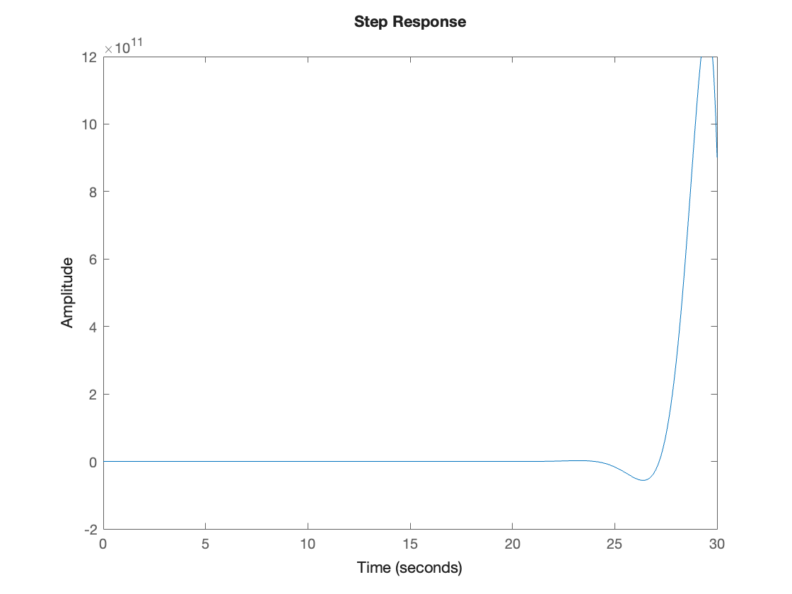
Bonus: the step response is

step(Fs)

../_images/f2d9b59500fe17dfac4cf1b3b85aa814cce4af2ac5de56eab9abdd06f5bd210d.png

Exercise 16.3: Spring-Mass-Damper System#

You can analyze a mass-spring-damper system (Fig. 81) by looking at the poles of its transfer function.

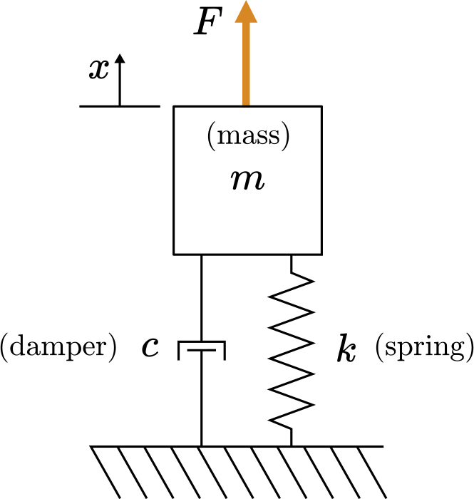
Fig. 81 Diagram of a spring-mass-damper system#

Consider a mass-spring-damper that

is dynamically forced by an arbitrary function
has zero initial conditions: $x (0) = 0$ and $x^{'} (0) = 0$

The position transfer function is

G (s) = \frac{X (s)}{U (s)} = \frac{1}{m s^{2} + c s + k}

(a) Write the mass-spring-damper transfer function in the form

G (s) = \frac{K}{s^{2} + 2 ζ ω_{n} s + ω_{n}^{2}}

and solve for the expressions of the gain $K$ , damping ratio $ζ$ , and natural frequency $ω_{n}$ in terms of the mass-spring-damper parameters. Write your answers using the symbolic variables $c$ , $m$ , and $k$ .

% Use these symbolic variables
syms m c k
% Replace the NaNs with your expressions
K = 1/m
omega_n = sqrt(k/m)
zeta = (c/m)/(2*omega_n)

K = \frac{1}{m}

o m e g a_{n} = \sqrt{\frac{k}{m}}

z e t a = \frac{c}{2 m \sqrt{\frac{k}{m}}}

(b) Solve for the symbolic expressions of the poles of $G$ in terms of the mass-spring-damper parameters $m$ , $c$ , and $k$ . Store the expressions below in pplus and pminus where pplus stores the positive root.

% Your solution here
poles = solve(s^2 + (c/m)*s + (k/m) == 0);
pplus = poles(1), pminus = poles(2)

p p l u s = - \frac{c - \sqrt{c^{2} - 4 k m}}{2 m}

p m i n u s = - \frac{c + \sqrt{c^{2} - 4 k m}}{2 m}

(c) Plot the step response of the system $G$ starting with $k = m = c = 1$ . Note the values of the poles, damping ratio, and natural frequency obtained. Observer the performance parameters returned by stepinfo. Adjust the values of $k$ , $m$ and $c$ and comment on the effects on the step response observed.

k = 1; m = 1; c = 1;
Gs = tf(1/m, [1 c/m k/m])

Gs

  -----------

  s^2 + s + 1

Continuous-time transfer function.

step(Gs)

../_images/3e21683f3640ff7e24b0e0f267b4f422d7ae97389e25dca8301fde11d6b395b6.png

p = pole(Gs)

p = 
  -0.5000 + 0.8660i
  -0.5000 - 0.8660i

[Wn,Z]=damp(Gs)

Wn = 2×1 double
    1.0000
    1.0000

Z = 2×1 double
    0.5000
    0.5000

stepinfo(Gs)

ans = struct with fields:
         RiseTime: 1.6390
    TransientTime: 8.0759
     SettlingTime: 8.0759
      SettlingMin: 0.9315
      SettlingMax: 1.1629
        Overshoot: 16.2929
       Undershoot: 0
             Peak: 1.1629
         PeakTime: 3.5920

Summary#

Unit 5.2: Take aways#

Real pole $s = σ$ :#

Growth rate: $σ > 0$ , the exponential signal doubles every $T \approx 0.7 / σ$ s.
Time constant: $σ < 0$ , the exponential signal decays to $37 %$ of it’s original value in $τ = 1 / σ$ s. The exponential signal reaches $1 %$ of it’s original value in $t \approx 4.6 τ$ s.

Complex pole pair $s = - σ \pm j ω$ :#

Representation of denominator: $(s + σ + j ω_{n}) (s - σ + j ω) = s^{2} + 2 σ s + (σ^{2} + ω_{n}^{2})$
Natural frequency: $ω_{n} = \sqrt{σ^{2} + ω^{2}}$
Damping ratio: $ζ = - σ / \sqrt{σ^{2} + ω^{2}}$

Standard second-order system transfer function#

Transfer function:

G (s) = \frac{K}{s^{2} + 2 ζ ω_{n} s + ω_{n}^{2}}

Poles: $p_{1, 2} = - ζ ω_{n} \pm j ω_{n} \sqrt{1 - ζ^{2}}$

Performance parameters for second-order system#

Rise time: $T_{r}$ is estimated from graph of normaized rise-time $ω_{n} T_{r}$ v $ζ$ shown in Fig. 80.
2% Setting time: $T_{s} \approx 4 / σ$
Percentage overshoot: $% OS = \exp (- ζ π / \sqrt{1 - ζ^{2}}) \times 100$
Peak time: $T_{p} = π / ω$

Useful MATLAB commands#

tf: defines a system as a transfer function $n (s) / d (s)$
step: plots the step response of a system
pole: lists the poles of a system
damp: lists the natural frequency and damping ratios of the poles of a system
stepinfo: lists the properties of the step response of a system

Unit 5.2: Further exploration#

If you have access to MATLAB (desktop of online), you can install the MATLAB curriculum module Transfer Function Analysis of Dynamic Systems [Allie, 2024] and further explore the concepts given here. The MATLAB Live Script PoleZeroAnalysis.mlx provides some interactive tools that enable you to interactively explore second order system response and includes the impact of zeros which we have not covered here.

References#

[All24] (1,2)

Chad Allie. Transfer function analysis of dynamic systems. 2024. Retrieved April 3, 2024. URL: MathWorks-Teaching-Resources/Transfer-Function-Analysis-of-Dynamic-Systems.

[Boy93]

Stephen Boyd. Ee-102: introduction to signals and systems. 1993. Retrieved April 3, 2024. URL: https://web.stanford.edu/~boyd/ee102/.

Unit 5.2: More on the Qualitative and Quantitative Response of First- and Second-Order Poles

Contents

Unit 5.2: More on the Qualitative and Quantitative Response of First- and Second-Order Poles#

Acknowledgements#

Agenda#

Quantitative behaviour of real poles#

Rate of exponential growth#

Example 7#

Solution to example 7#

Rate of exponential decay#

Example 8#

Solution to example 8#

Natural frequency#

Analysis of a second-order system#

Pole analysis#

Natural response#

Step-response of a second-order system#

Example 9#

Solution to example 9#

Useful quantifiers that result from step response#

Poles#

Damping ratio and natural frequencies#

Rise-time#

Settling time#

Peak overshoot#

Peak time#

List all properties#

Exercises 16#

Exercise 16.1: Qualitative analysis#

Exercise 16.2: Qualitative and quantitative analysis#

Partial solution to Exercise 16.2#

Exercise 16.3: Spring-Mass-Damper System#

Summary#

Unit 5.2: Take aways#

Real pole s=σ:#

Complex pole pair s=−σ±jω:#

Standard second-order system transfer function#

Performance parameters for second-order system#

Useful MATLAB commands#

Unit 5.2: Further exploration#

References#

Real pole $s = σ$ :#

Complex pole pair $s = - σ \pm j ω$ :#