Unit 3.3: Systems Described by Differential Equations#
This section is based on Section 2.5 of [Hsu, 2020]
Follow along at cpjobling.github.io/eg-150-textbook/lti_systems/lti3

Subjects to be covered#
We conclude our introduction to continuous-time LTI system by considering
Continuous-time LTI systems described by differential equations#
A. Linear constant-coefficient differential equations#
A general \(N\)th-order linear constant-coefficient ordinary differential (LCCODE) equation is given by
where the coeeficients \(a_k\) and \(b_k\) are real constants and usually \(N > M\).
The order \(N\) refers to the highest derivative of \(y(t)\) in the differential equation.
The LCCODE can be written in more compact form as
Applications of linear constant-coefficient differential equations#
LCCODEs play a central role in describing the input-output relationships of a wide variety of electrical, mechanical, chemical and biological systems.
Illustration: An RC Circuit#
For instance, in the RC circuit considered in Exercise 4.1: RC Circuit, the input \(x(t)=v_s(t)\) and the output \(y(t)=v_c(t)\) are related by a first-order constant-coefficient differential equation
So, by inspection, \(N=1\), \(a_1 = 1\), \(a_0 = b_0 = 1/RC\).
General solution of the general linear constant-coefficient differential equation#
The general solution of the general linear constant-coefficient differential equation for a particular input \(x(t)\) is given by
where \(y_p(t)\) is a particular solution satisfying the linear constant-coefficient differential equation and \(y_h(t)\) is a homegeneous solution (or complementary solution) satisfying the homegeneous differential equation
The exact form of \(y_h(t)\) is determined by \(N\) auxiliary conditions.
Note that
does not completely specify the the output \(y(t)\) in terms of \(x(t)\) unless auxiliary conditions are defined. In general. a set of auxiliary conditions are the values of
at some point in time.
B. Linearity#
The system defined by
will be linear only if all the auxilliary conditions are zero (see Exercise 8.4).
If the auxilliary conditions are not zero, then the response \(y(t)\) of a system can be expressed as
where \(y_\mathrm{zi}(t)\) called the zero-input response, is the response to the aunxilliary conditions, and \(y_\mathrm{zs}(t)\), called the zero-state response, is the response of a linear system with zero auxiliary conditions.
This is illustrated in Fig. 38
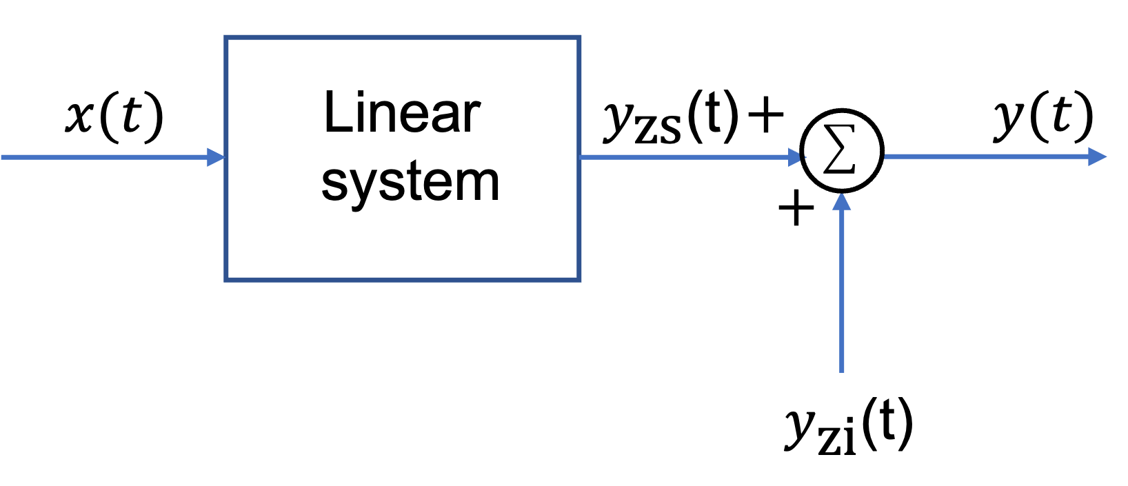
Fig. 38 Zero-state and zero-input responses#
Note that \(y_\mathrm{zi}(t) \neq y_h(t)\) and \(y_\mathrm{zs}(t) \neq y_p(t)\) and that in general \(y_\mathrm{zi}(t)\) contains \(y_h(t)\) and \(y_\mathrm{zs}(t)\) contains both \(y_h(t)\) and \(y_p(t)\) (see Exercise 8.3).
C. Causality#
In order for the linear system described by a linear constant-coefficient differential equation
to be causal, we must assume the condition of initial rest (or an initially relaxed condition).
That is, if \(x(t)=0\) for \(t\le t_0\), then assume \(y(t) = 0\) for \(t\le t_0\) (See Exercise 4.6).
Thus, the response for \(t > t_0\) can be calculated from the linear constant-coefficient differential equation with the initial conditions
where
Clearly, at initial rest, \(y_\mathrm{zs}(t)=0\).
D. Time-invariance#
For a linear causal system, initial rest also implies time-invariance (Exercise 8.6).
E. Impulse response#
The impulse response \(h(t)\) of a linear constant-coefficient differential equation satisfies the differential equation
with the initial rest condition.
Examples of finding impulse responses are given in Exercise 8.6 to Exercise 8.8.
A peek into the future#
Later in this course, and probably for the rest of your career, you will find the impulse and other responses by using the Laplace transform.
Exercises 8: Systems described by differential equations#
Exercise 8.1#
The continuous-time system shown in Fig. 39 consists of one integrator and one scalar multiplier. Write the differential equation that relates the output \(y(t)\) to the input \(x(t)\).
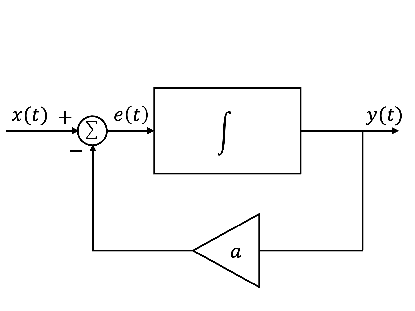
Fig. 39 A one-integrator linear system#
For the answer, refer to the lecture recording or see solved problem 2.18 in [Hsu, 2020].
MATLAB Solution#
cd '/Users/eechris/code/src/github.com/cpjobling/eg-150-textbook/lti_systems/matlab'
open examples8
You can download and run these scripts and try them yourself.
MATLAB Scipt examples8.slx
Simulation model example8_1.slx
Exercise 8.2#
The continuous-time system shown in Fig. 40 consists of two integrators and two scalar multipliers. Write the differential equation that relates the output \(y(t)\) to the input \(x(t)\).
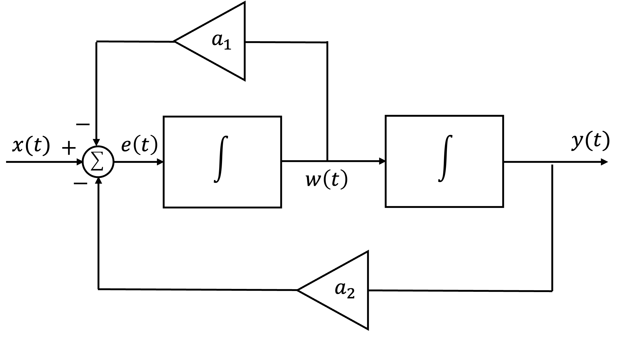
Fig. 40 A two-integrator linear system#
For the answer, refer to the lecture recording or see solved problem 2.19 in in [Hsu, 2020].
MATLAB Solution#
Simulink model example8_2.slx
Note
As we will be moving on to show how differential equations can be solved by the Laplace transform, the remaining examples are optional and will not be examined.
Exercise 8.3#
Consider a continuous-time system whose input \(x(t)\) and output \(y(t)\) are related by
where \(a\) is a constant.
(a) Find \(y(t)\) with the auxilliary condition \(y(0) = y_0\) and
(b) Express \(y(t)\) in terms of the zero-input and zero-state responses.
Solution#
This is an example of how a first-order LCCODE would be solved. We provide this as an instructional example but will assume that you will be tested on this in other modules.
a) Given that
we assume that the particular solution will be of the form \(y_p(t) = Ae^{-bt}\).
Substituting for \(y_p(t)\) in the differential equation we have
from which, after cancelling the common term \(e^{-bt}\), gives
and
To obtain the homegenous solution we assume that
Substituting for \(y_h(t)\) in the differential equation we have
so \(s=-a\) and
Combining \(y_p(t)\) and \(y_h(t)\) we have
Using the auxilary equation \(y(0) = y_0\)
then
For \(t < 0\) we have \(x(t) = 0\) and the differential equation becomes equal to the homogeneous equation \(y_h(t)\) so
From the auxillary equation \(y(0) = y_0\), we obtain
b) Combining the solutions for \(y(t) > 0\) and \(y(t) < 0\), y(t) can be expression in terms of \(y_\mathrm{zi}(t)\) (zero-input response and \(y_\mathrm{zs}(t)\) (zero-state response) as
where
and
Exercise 8.4#
Consider the system in Exercise 8.3.
(a) Show that the system is not linear if \(y(0)=y_0\neq 0\).
(b) Show that the system is linear if \(y(0) = 0\).
For the answer, see the solved problem 2.21 in [Hsu, 2020].
Exercise 8.5#
Consider the system in Exercise 8.3. Show that the initial rest condition \(y(0) = 0\) also implies that the system is time-invariant.
For the answer, see the solved problem 2.22 in [Hsu, 2020].
Exercise 8.6#
Consider the system in Exercise 8.3. Find the impulse response \(h(t)\) of the system.
For the answer, see the solved problem 2.23 in [Hsu, 2020].
Exercise 8.7#
Consider the system in Exercise 8.3 with \(y(0)=0\).
(a) Find the step response \(s(t)\) of the system without using the impulse response \(h(t)\).
(b) Find the step response \(s(t)\) of the system with the impulse response \(h(t)\) obtained in Exercise 8.6.
(c) Find the impulse response \(h(t)\) from the step response \(s(t)\).
For the answer, see the solved problem 2.24 in [Hsu, 2020].
Exercise 8.8#
Consider the system described by
Find the impulse response \(h(t)\) of the system.
For the answer, refer to the lecture recording or see solved problem 2.25 in [Hsu, 2020].
Summary#
In this lecture we have concluded our introduction to LTI systems by looking at linear constant-coefficient differential equations.
Unit 3.3: Take aways#
LCCODEs#
Continuous-time LTI systems are often modelled as linear constant coefficient ordinary differential equations (LCCODEs). The solution of such equations has wide application in engineering and science.
The general description of a LCCODE is given in compact form as:
where the coefficients \(a_k\) and \(b_k\) are real constants and \(n\) and \(m\) are integers.
We illustrated in Illustration: An RC Circuit that the simple RC circuit can be represented as such an LCCODE.
Solution of LCCODEs#
The solution of LCCODEs requires the determination and combination of the homegenious solution which is due only to the output \(y(t)\) and its derivatives, and a particular solution which takes account of the input \(x(t)\), its derivatives, and the initial values of \(y(t)\) and its derivatives.
We were told that continuous-time LTI systems defined by LCCODEs are only causal and time invariant if they are initially at rest.
The output of the continuous-time LTI system with input \(x(t)\) that is at rest and has zero initial conditions is called the zero-state output \(y_\mathrm{zs}(t)\). The outputs due to the inital conditions can be computed from the system with zero input which is named \(y_\mathrm{zi}(t)\). The total response of such a system is given by \(y(t) = y_\mathrm{zs}(t) + y_\mathrm{zi}(t)\).
For reference, a fully worked solution of a first-order LCCODE is provided in Exercise 8.3. You will not be expected to solve such problems in the assessments for this module.
Analogue computer models#
In Exercises 8: Systems described by differential equations we were introduced to the representation of an LCCODE as a block diagram constructed from integral, gain and summing blocks. Such models were the basis of analogue computation which was used widely by engineers before the widespread adoption of digital computers. Models based on integration are still the basis of modern numerical digital system simulation tools like Multisim and Simulink.
Examples of the solution of Exercise 8.1 and Exercise 8.2 have been provided in MATLAB and Simulink.
Looking ahead#
Any continuous-time LTI system that can be represented by an LCCODE can be solved by taking the Laplace transform of the differential equation. The derivative terms like \(a_k d^n y(t)/dt^n\) become polynomial terms like \(a_k s^n Y(s)\), where \(Y(s)\) is the Laplace transform of \(y(t)\). As we shall see in unit4, such systems are then representable as rational polynomials in \(s\) and are easily solved using algebraic techniques such as polynomial factorization and partial fraction expansion.
Continuous-Time LTI Systems Described by Differential Equations#
Next Time#
We move on to consider