Unit 4.7: Transfer Functions for Circuit Analysis#
The preparatory reading for this section is Chapter 4.4 [Karris, 2012] which discusses transfer function models of electrical circuits. We have also adapted content from 3.6 The System Function from [Hsu, 2020].
Follow along at cpjobling.github.io/eg-150-textbook/laplace_transform/7/tf_for_circuits

Agenda#
In this unit, we will explore how transfer functions introduced in Unit 4.6: Transfer Functions can be applied to the analysis of circuits.
% Initialize MATLAB
clearvars
cd ../matlab
format compact
Transfer Functions for Circuits#
When doing circuit analysis with components defined in the complex frequency domain, the ratio of the output voltage \(V_{\mathrm{out}}(s)\) to the input voltage \(V_{\mathrm{in}}(s)\) under zero initial conditions is of great interest.
This ratio is known as the voltage transfer function denoted \(G_v(s)\):
Similarly, the ratio of the output current \(I_{\mathrm{out}}(s)\) to the input current \(I_{\mathrm{in}}(s)\) under zero initial conditions, is called the current transfer function denoted \(G_i(s)\):
In practice, the current transfer function is rarely used, so we will use the voltage transfer function denoted:
Exercises 14#
We will work through these and demonstrate the MATLAB solutions in class.
Exercise 14.1#
Derive an expression for the transfer function \(G(s)\) for the circuit shown in Fig. 68.
In this circuit \(R_g\) represents the internal resistance of the applied (voltage) source \(v_s\), and \(R_L\) represents the resistance of the load that consists of \(R_L\), \(L\) and \(C\).
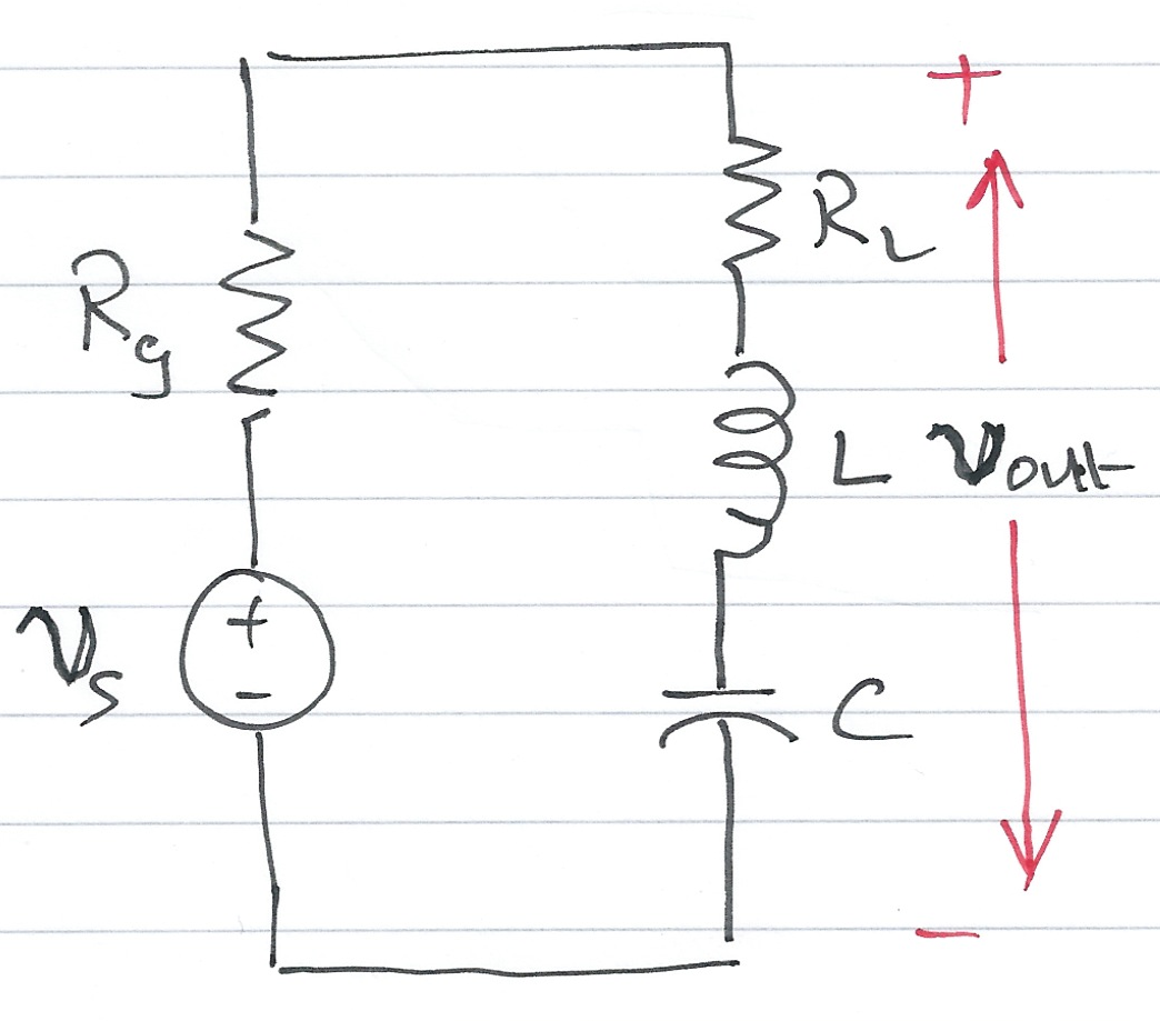
Fig. 68 Circuit for Example 14.1#
Sketch of Solution for Example 14.1#
Replace \(v_s(t)\), \(R_g\), \(R_L\), \(L\) and \(C\) by their transformed (complex frequency) equivalents: \(V_s(s)\), \(R_g\), \(R_L\), \(sL\) and \(1/(sC)\)
Use the Voltage Divider Rule to determine \(V_\mathrm{out}(s)\) as a function of \(V_s(s)\)
Form \(G(s)\) by writing down the ratio \(V_\mathrm{out}(s)/V_s(s)\)
Have a go for the next five minutes.
Worked solution for Example 14.1#
Pencast: ex6.pdf - open in Adobe Acrobat Reader.
Answer for Example 14.1#
Exercise 14.2#
MATLAB Example
This is based on Example 4.7 from [Karris, 2012].
This is the basis for the mini project in MATLAB Lab 5.
Compute the transfer function for the op-amp circuit shown in Fig. 69 in terms of the circuit constants \(R_1\), \(R_2\), \(R_3\), \(C_1\) and \(C_2\).
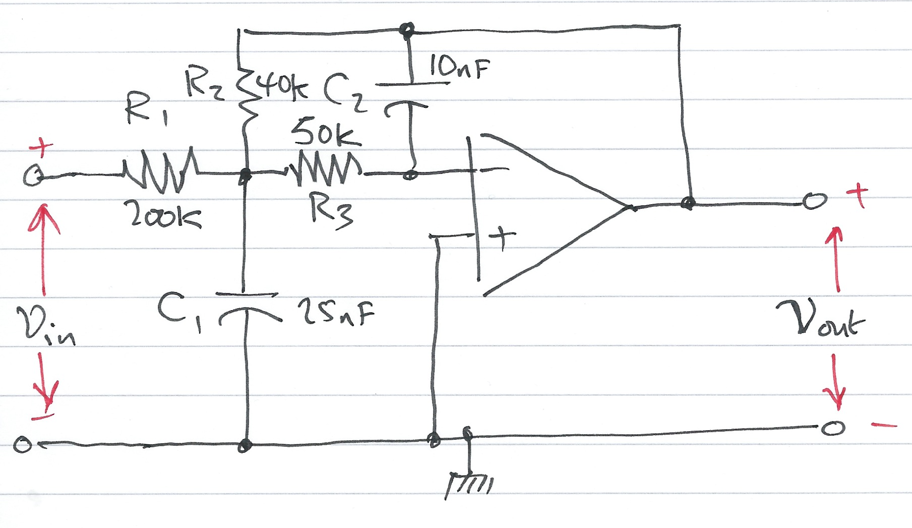
Fig. 69 OpAmp circuit for Example 14.2#
Then replace the complex variable \(s\) with \(j\omega\), and the circuit constants with their numerical values and plot the magnitude
versus radian frequency \(\omega\) rad/s.
Sketch of Solution for Example 14.2#
Replace the components and voltages in the circuit diagram with their complex frequency equivalents
Use nodal analysis to determine the voltages at the nodes either side of the 50K resistor \(R_3\)
Sketch of Solution for Example 14.2 (continued)#
Note that the voltage at the input to the op-amp is a virtual ground
Solve for \(V_{\mathrm{out}}(s)\) as a function of \(V_{\mathrm{in}}(s)\)
Form the reciprocal \(G(s) = V_{\mathrm{out}}(s)/V_{\mathrm{in}}(s)\)
Have a go for the next five minutes
Answer for Example 14.2#
Worked solution for Example 14.2#
Pencast: ex7.pdf - open in Adobe Acrobat Reader.
Sketch of Solution for Example 14.2 (continued)#
Use MATLAB to calculate the component values, then replace \(s\) by \(j\omega\).
Compute \(\left|G(j\omega)\right|\) and plot on log-linear “paper”.
The MATLAB Bit#
Set up the symbols we will be using. In this case just the Laplace complex frequency \(s\).
syms s
Now define the values of the components
R1 = 200*10^3; % 200 kOhm
R2 = 40*10^3;  %  40 kOhm
R3 = 50*10^3;  %  50 kOhm

C1 = 25*10^(-9); % 25 nF
C2 = 10*10^(-9); % 10 nF
Define the transfer function derived from analysis (Eq. (41))
den = R1*((1/R1+ 1/R2 + 1/R3 + s*C1)*(s*R3*C2) + 1/R2)
Simplify coefficients of \(s\) in the denominator. Note sym2poly converts a symbolic polynomial with numerical coeficients into a MATLAB polynomial.
format long
denH = sym2poly(den)
denH = 1×3 double
   0.000002500000000   0.005000000000000   5.000000000000000
Now define the numerator
numH = -1;
Plot the frequency response
For convenience, define coefficients \(a\) and \(b\):
a = denH(1)
b = denH(2)
a = 2.500000000000000e-06
b = 0.005000000000000
w = 1:10:10000;
Hw = -1./(a*w.^2 - j.*b.*w + denH(3));
Plot \(|H(j\omega)|\) against \(\omega\) on log-lin “graph paper”.
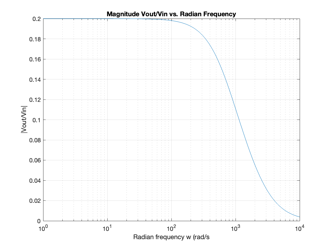
semilogx(w, abs(Hw))
xlabel('Radian frequency w (rad/s')
ylabel('|Vout/Vin|')
title('Magnitude Vout/Vin vs. Radian Frequency')
grid
Note
Note that this is a low-pass filter. Sinusoids at low frequencies are passed with a gain of 0.2. For frequencies above around 100 rad/s, the filter starts to increase the attenuation of the passed signal. At 10,000 rad/s, the attenuation is 1/10 of the attenuation at 1,000 rad/s.
MATLAB Solutions#
For convenience, single script MATLAB solutions to the examples are provided and can be downloaded from the accompanying MATLAB folder.
open example_14_2
Summary#
In this unit, we will explored how transfer functions introduced in Unit 4.6: Transfer Functions can be applied to the analysis of circuits.
Unit 4.7: Take Away#
The ratio of the output voltage \(V_\mathrm{out}(s)\) to the input voltage \(V_\mathrm{in}(s)\) under zero initial conditions is of great interest. We call this ratio the voltage transfer function
We can consider other ratios such as the current transfer function
but in practice this is rarely used.
Next time#
We explore the facilties provided by other toolboxes in MATLAB, most notably the Control Systems Toolbox and the simulation tool Simulink in Unit 4.8: Computer-Aided Systems Analysis and Simulation. We will also look at some of the problems you have studied in EG-152 Analogue Design hopefully confirming some of the results you have obbserved in the lab.
References#
Hwei P. Hsu. Schaums outlines signals and systems. McGraw-Hill, New York, NY, 2020. ISBN 9780071634724. Available as an eBook. URL: https://www.accessengineeringlibrary.com/content/book/9781260454246.
Steven T. Karris. Signals and systems with MATLAB computing and Simulink modeling. Orchard Publishing, Fremont, CA., 2012. ISBN 9781934404232. Library call number: TK5102.9 K37 2012. URL: https://ebookcentral.proquest.com/lib/swansea-ebooks/reader.action?docID=3384197.