Unit 4.1: The Laplace Transformation#
The preparatory reading for this section is Chapter 2 of [Karris, 2012] and Chapter 3 of [Hsu, 2020].
Follow along at cpjobling.github.io/eg-150-textbook//laplace_transform/1/laplace

In this unit we will present the Laplace transform and look at some important properties that go with it.
Agenda#
The Laplace Transform#
In Eigenfunctions of Continuous-Time LTI Systems we saw that for a continuous-time LTI system with impulse response \(h(t)\), the output of the system in response to a complex input of the form \(x(t)=e^{st}\) is
where
Definition#
The function \(H(s)\) above is referred to as the Laplace transform of \(h(t)\).
For a general continuous-time signal \(x(t)\), the Laplace transform \(X(s)\) is defined as
The variable \(s\) is generally complex valued and is expressed as
The Laplace transform defined above is often called the bilateral (or two-sided) Laplace transform in contrast the the unilateral (or one-sided) Laplace transform which is defined as
where \(0^-=\lim_{\epsilon\to 0}(0-\epsilon)\).
Clearly the bilateral and unilateral tranforms are equivalent only if \(x(t)=0\) for \(t\lt 0\).
In this course, because we are dealing with causal signals and systems, we will be concerned only with unilateral Laplace transform.
The laplace tranform equation is sometimes considered an operator that transforms a signal \(x(t)\) into a function \(X(s)\) represented symbolically as
and the signal \(x(t)\) and its Laplace transform \(X(s)\) are said to form a Laplace transform pair denoted as
Laplace transform pairs are tabulated (Common Laplace Transform Pairs) for ease of reference.
Note
By convention, lower-case symbols are used for continuous-time signals and uppercase symbols for their Laplace tranforms.
MATLAB Representation#
The Laplace transform operator is provided in the MATLAB symbolic math toolkit by the function laplace and can be used as follows:
% set up
format compact
%setappdata(0, "MKernel_plot_format", 'svg')
syms s t x(t) % define Laplace transform variable and time as symbols
X(s) = laplace(x(t))
Region of Convergence#
For a Laplace transfomation to exist, the integral must be bounded. That is
The range of values for the complex variables \(s\) for which the Laplace tranform converges is called the region of convergence (ROC). To illustrate this concept, let us consider some examples.
Solved Problem 1#
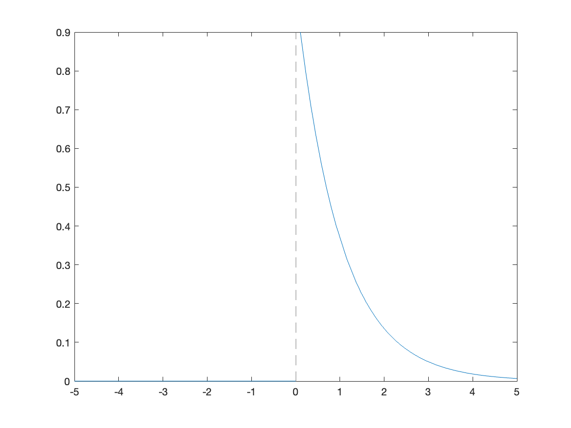
Consider the signal
By hand#
We will work through the analysis in class.
MATLAB analysis#
syms s t a
assume(a,'real')
u0(t) = heaviside(t);
x(t) = exp(-a*t)*u0(t)
fplot(subs(x(t),a,1))
int(x(t)*exp(-s*t),t,0,inf)
assume(s + a > 0)
int(x(t)*exp(-s*t),t,0,inf)
X(s) = laplace(x(t))
The Laplace transform of \(x(t)\)
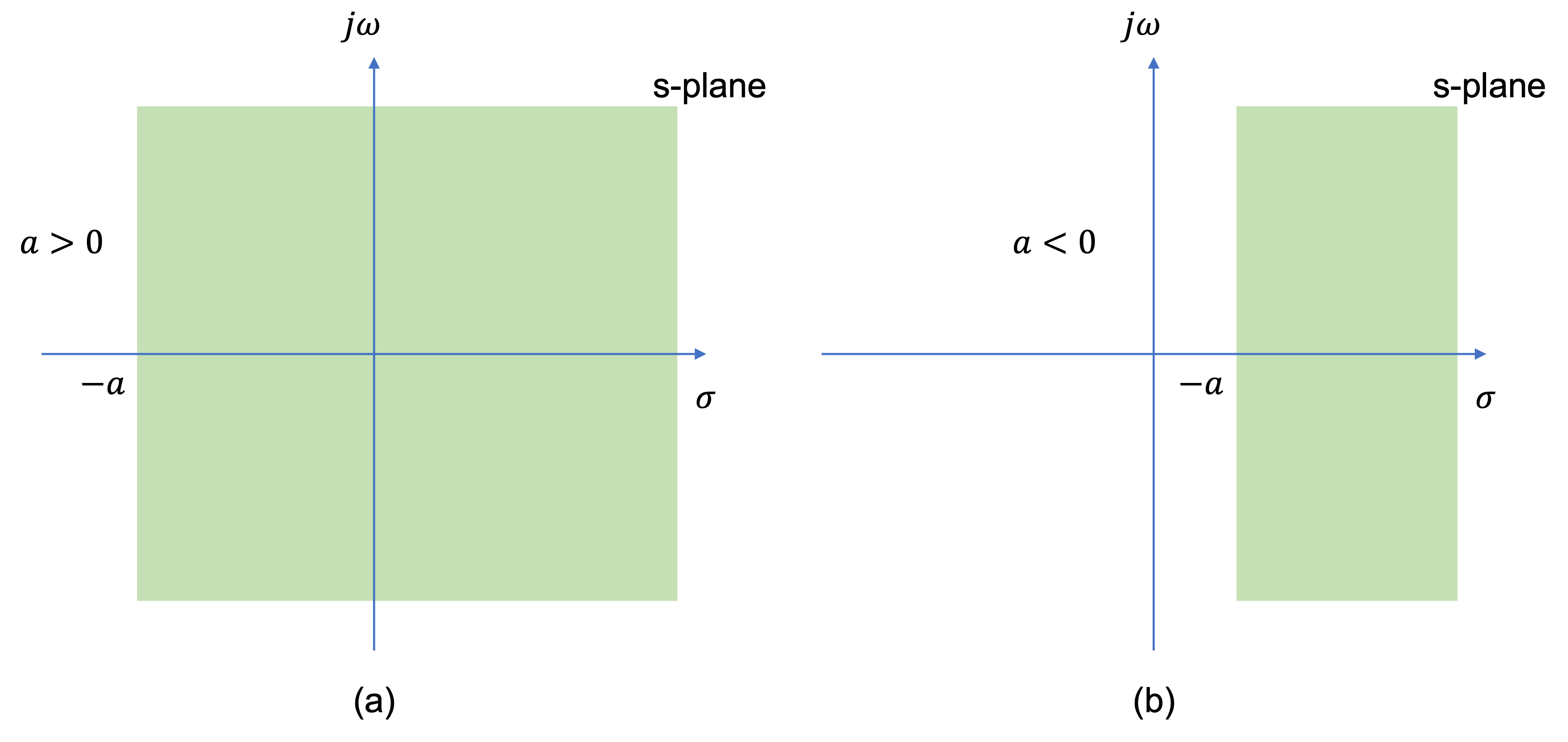
Fig. 42 ROC for Example 1#
because \(\lim_{t\to \infty}e^{-(s+a)t} = 0\) only if \(\mathrm{Re}(s + a)\gt 0\) or \(\mathrm{Re}(s)\gt -a\).
Thus, the ROC for Solved Problem 1 is specified as \(\mathrm{Re}(s)\gt -a\) and is illustrated in the complex plane as showm in Fig. 43 by the shaded area to the right of the line \(\mathrm{Re}(s)=-a\).
In Laplace transform applications, the complex plane is commonly referred to as the s-plane. The horizontal and vertical axes are sometimes referred to as the \(\sigma\)-axis (\(\mathrm{Re}(s)\)) and the \(j\omega\)-axis (\(\mathrm{Im}(s)\)), respectively.
Solved Problem 2#
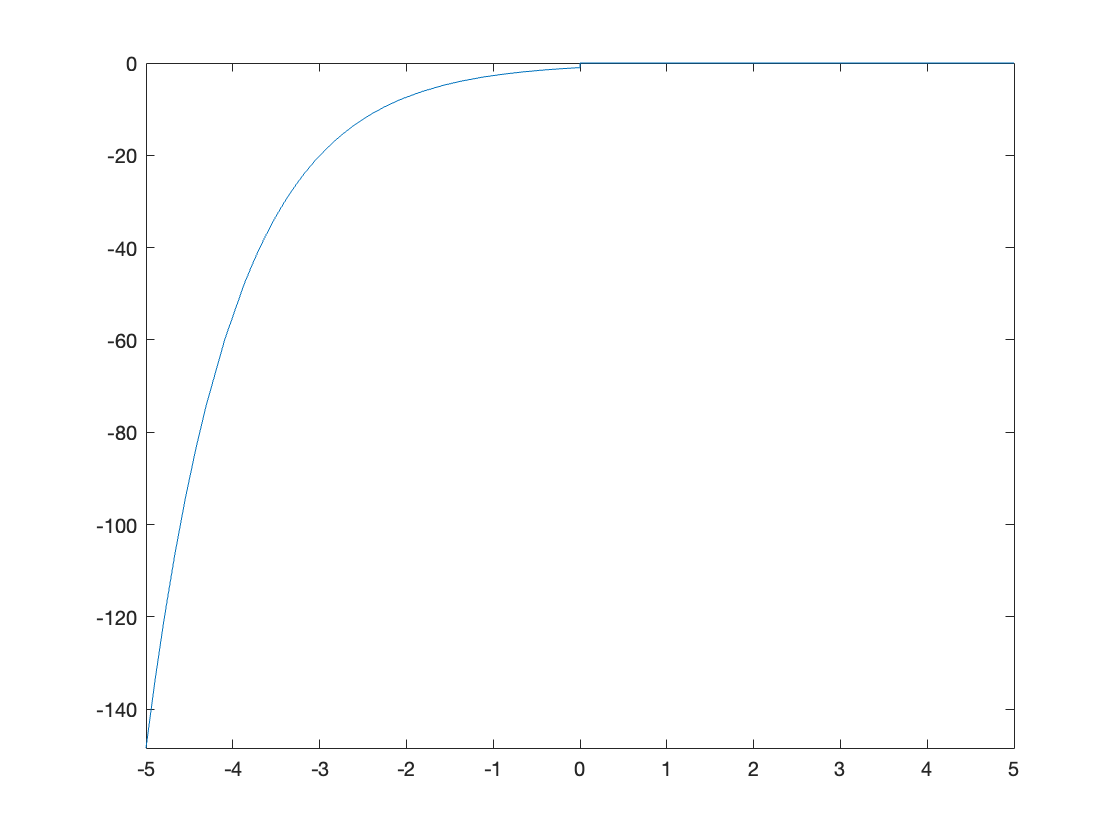
Consider the signal
MATLAB Analysis#
We will work through the analysis in class
x(t) = -exp(-a*t)*u0(-t)
fplot(subs(x(t),a,1))
int(x(t)*exp(-s*t),t,-inf,0)
X(s)=laplace(x(t))
assume(s + a < 0)
int(x(t)*exp(-s*t),t,-inf,0)
By hand analysis#
See ex9.1.
Its Laplace transform \(X(s)\) is given by Exercise 9.1
Thus the ROC for Solved Problem 2 is specified as \(\mathrm{Re}(s)\lt -a\) and is illustrated in the complex plane as shown in Fig. 43 by the shaded area to the left of the line \(\mathrm{Re}(s)=-a\).
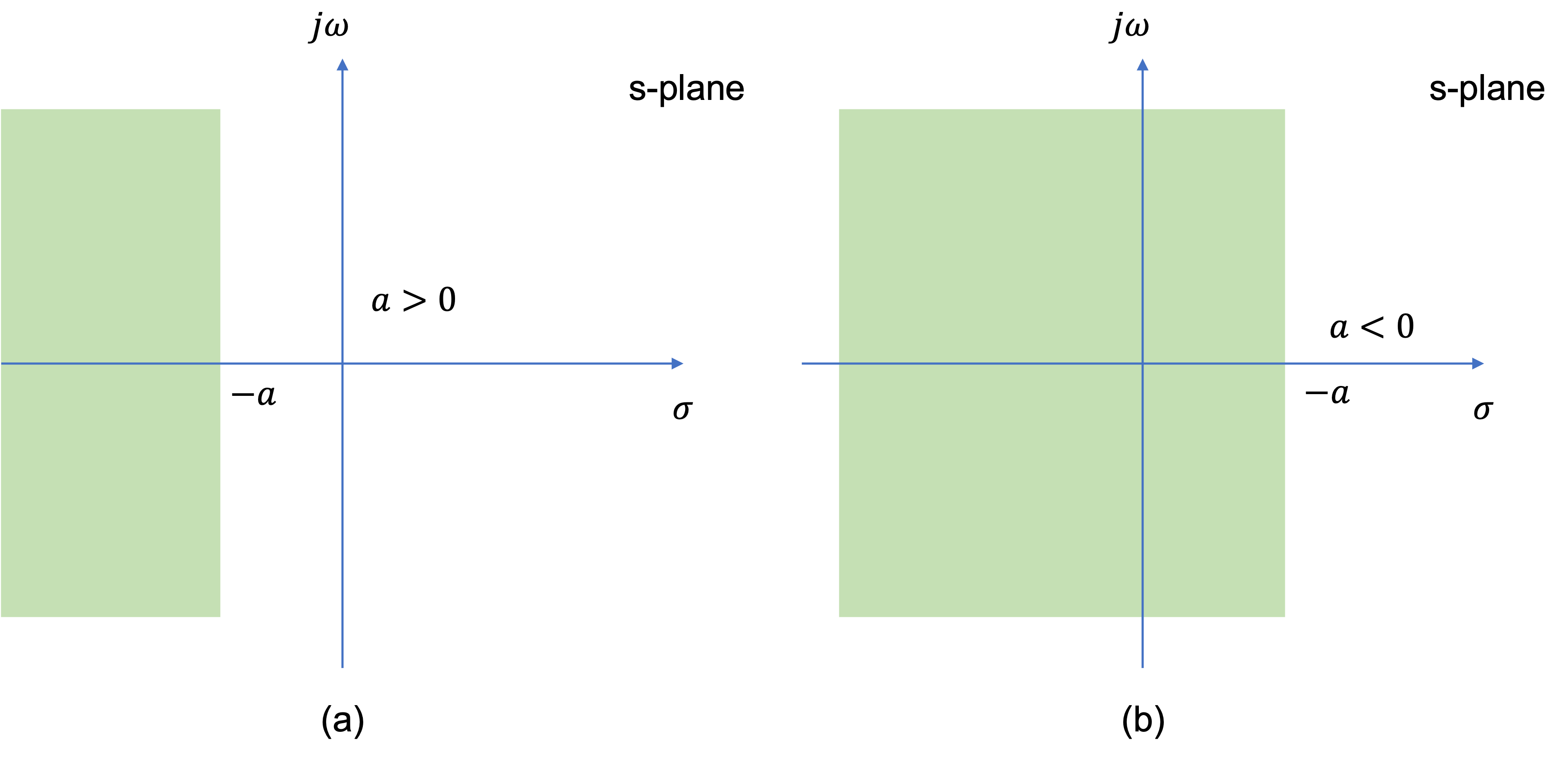
Fig. 43 ROC for Example 2#
Comparing the results of Solved Problem 1 and Solved Problem 2, we see that that algebraic expressions for \(X(s)\) for these two signals are identical apart from the ROCs.
Therefore, in order for the Laplace transform to be unique for each signal \(x(t)\), the ROC must be specified as part of the transform.
Poles and Zeros of X(s)#
Usually, \(X(s)\) will be a rational polynomial in \(s\); that is
The coefficients \(b_k\) and \(a_k\) are real constants, and \(k\), \(m\) and \(n\) are positive integers.
The transform \(X(s)\) is called a proper rational function if \(n>m\), and an improper rational function if \(n\le m\).
The roots of the numerator polynomial, \(z_k\), are called the zeros of \(X(s)\) because \(X(s) = 0\) for those values of \(s\).
Similarly, the zeros of the denominator polynomial, \(p_k\), are called the poles of \(X(s)\) because \(X(s)\) is infinite for those values of \(s\).
Therefore, the poles of \(X(s)\) lie outside the ROC since, by definition, \(X(s)\) does not converge on the poles.
The zeros, on the other hand, may lie inside or outside the ROC.
Except for the scale factor \(b_m/a_n\), \(X(s)\) can be completely specified by its poles and zeros.
Thus a very compact representation of \(X(s)\) is the s-plane is to show the locations of the poles and zeros in addition to the ROC.
Traditionally, an “x” is used to indicate each pole and a “o” is used to indicate each zero.
This is illustrated in Fig. 44 for \(X(s)\) given by
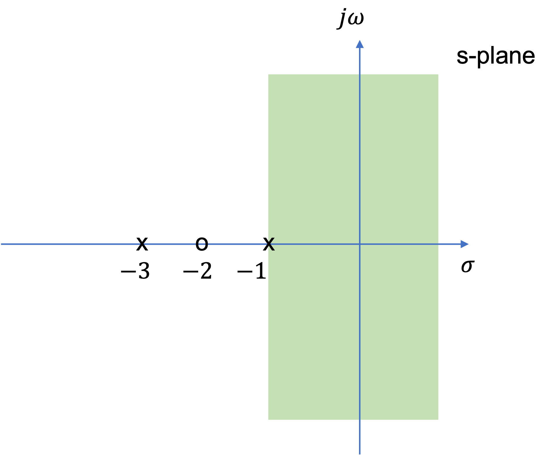
Fig. 44 s-plane representation of \(X(s)=(2s^2+4)/(s^2+4s+3)\)#
MATLAB Analysis#
In MATLAB we represent polynomials as vectors whose elements are the numerical values of the coeffients in decending order of \(s\):
n = [2 4]; d = [1 4 3];
We factorise using function roots which determines the zeros of the polynomials:
z = roots(n), p = roots(d), k = 2;
z = -2
p = 2×1 double
    -3
    -1
We can plot these on the \(s\)-plane using the function pzmap:
pzmap(p,z)
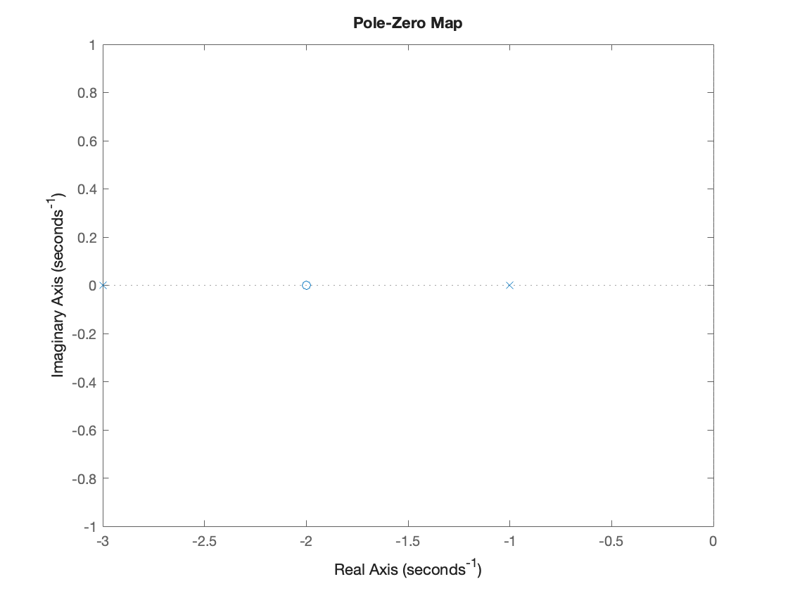
Note that \(X(s)\) has one zero at \(s=-2\) and two poles at \(s=-1\) and \(s=-3\) with scale factor 2. The ROC is \(\mathrm{Re}(s)>-1\).
Properties of the ROC#
[not examinable]
The properties of the ROC are summarised in Section 3.1 D of schaum and as they are not examinable, we leave their study to the interested student.
Exercises 9#
Exercise 9.1#
Find the Laplace transform of
a). \(x(t)=-e^{-at}u_0(-t)\)
b). \(x(t)= e^{at}u_0(-t)\)
Solution#
a)
Thus we obtain
b). Similarly
Thus we obtain
Summary#
In this unit we presented the Laplace transform and look at some important properties that go with it. The following topics were covered:
Unit 4.1: Takeaways#
The Laplace transform#
The Laplace transform of a continuous-time signal or system is defined as
The term \(s\) is called the complex frequency and is a complex number of form \(\sigma + j\omega\). The \(s\)-plane is a surface representing all the possible values of \(s\).
For causal signals and systems that are linear-time invariant, we will use the single-sided Laplace transform
Tunctions of time and their Laplace transforms are often presented using the transform-pair notation
Region of convergence#
The Laplace transform exists only if the integral is finite or
The region of the \(s\)-plane for which the Laplace transform is defined is called the Region of Convergence (ROC).
To be fully defined, the Laplace tranform of \(f(t)\) needs to specify the ROC. But in practice, for the systems and signals we are concerned about, we often neglect the ROC - although it is usually quoted in tables.
Poles and zeros#
For the signals and systems we are concerned about the Laplace transform takes the form of a rational polynomial in \(s\) which has the general form
where \(b_k\) and \(a_k\) are real constants, \(n\) and \(m\) are integers and \(n > m\).
The numerator and denominator polynomials can be factorised into the so-called zero-pole-gain form polynomial
The terms \(z_k\) which appear in the factors of the numerator polynomial and are called zeros (or roots) of the polynomial. (That is the values of \(s\) for which the numerator polynomial is zero.) The zeros of the numerator are also the zeros of the Laplace transform \(F(s)\).
The terms \(p_k\) which appear in the factors of the denominator polynomial and are called the poles of the laplace Transform. This is because any zeros in the denoniminator will result in infinities in the Laplace transform.
The poles and zeros will eaither be real or imaginary. If they are imaginary, they will appear as complex conjugate pairs and can be represented in the polynomial as quadratic factors \(s^2 + as + b\).
As we will see later, any function \(F(s)\) that has this structure can be expended using partial fractions and the response \(f(t)\) will be the sum of simple functions of time that can be readily looked up from tables.
The structure of any \(F(s)\) can be represented on the \(s\)-plane as a pole-zero map, and knowledge of the behaviour of the poles and the impact of the zeros allows us to reason about what the overal system response will look like. We will explore this later in the module and it will be an important topic of study in EG-243 Control Systems next year.
MATLAB#
The Laplace transform is available in the MATLAB Symbolic Math Toolbox as function laplace. To use it we usually specify the values t and s as symbols:
syms s t f(t)
F(s) = laplace(f(t))
Warning
The Laplace transform provided by MATLAB is single sided. If you need to find the laplace transform of a signal that is not causal, you need to define the region of convergence, and use the integral. See examples above.
The Laplace transform is representable in MATLAB using polynomials.
The roots of these polynomials can be determined using the roots function
Factored polynomials can be presented using the roots and the poles and zeros can be plotted on the \(s\)-plane using the pzmap function.
Example#
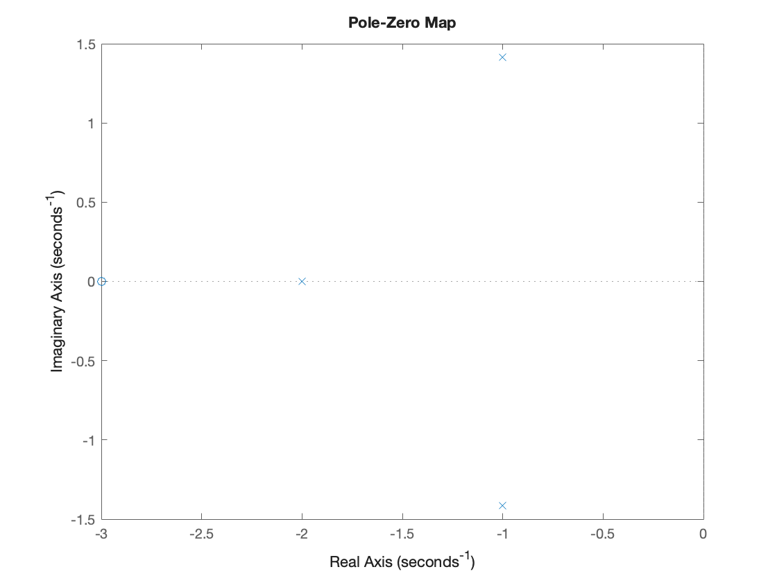
Factorise
and plot the pole-zero map
Nx = [3 9]; Dx = [1 4 7 6]; % coefficients in descending powers of s
Zeros = roots(Nx)
Poles = roots(Dx) % Note the roots are complex!
K = 3
pzmap(Poles,Zeros)
Zeros = -3
Poles =
  -2.0000 + 0.0000i
  -1.0000 + 1.4142i
  -1.0000 - 1.4142i
K = 3
Next Time#
We move on to consider
References#
Hwei P. Hsu. Schaums outlines signals and systems. McGraw-Hill, New York, NY, 2020. ISBN 9780071634724. Available as an eBook. URL: https://www.accessengineeringlibrary.com/content/book/9781260454246.
Steven T. Karris. Signals and systems with MATLAB computing and Simulink modeling. Orchard Publishing, Fremont, CA., 2012. ISBN 9781934404232. Library call number: TK5102.9 K37 2012. URL: https://ebookcentral.proquest.com/lib/swansea-ebooks/reader.action?docID=3384197.