Unit 4.5: Using Laplace Transforms for Circuit Analysis#
The preparatory reading for this section is Chapter 4 [Karris, 2012] which presents examples of the applications of the Laplace transform for electrical solving circuit problems. Much of the same material is covered in Section 3.7 D of [Hsu, 2020].
Follow along at cpjobling.github.io/eg-150-textbook/laplace_transform/5/circuit_analysis

Agenda#
We look at applications of the Laplace Transform for circuit analysis. In particular we will consider
Initialize MATLAB#
cd /Users/eechris/code/src/github.com/cpjobling/eg-150-textbook/laplace_transform/matlab/
clearvars
format compact
syms t L R C i_R(t) v_R(t) i_L(t) v_L(t) v_C(t) i_C(t)
Initialize for Slido Polling#
Open slido.com connect to session ID # 1205 320
Circuit Transformation from Time to Complex Frequency#
(resistive_network}=
Time Domain Model of a Resistive Network#
Consider Fig. 50
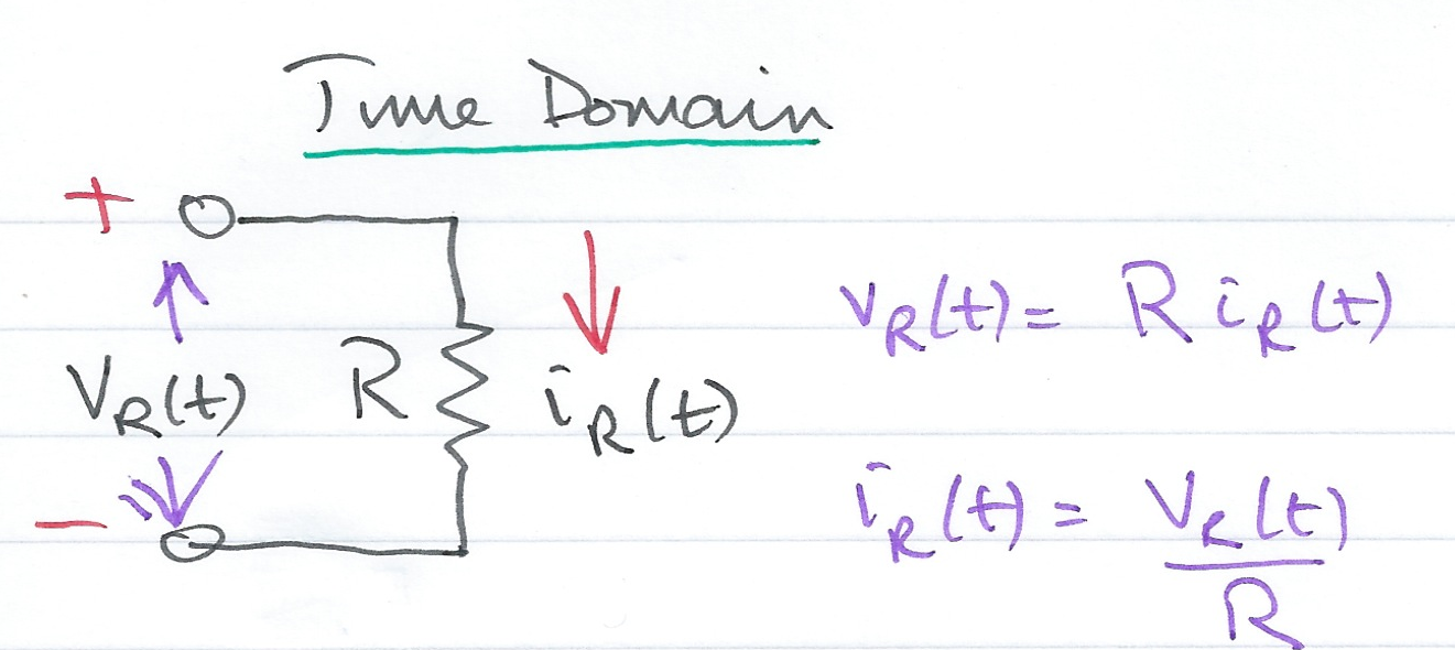
Fig. 50 Time Domain Model of a Resistive Network.#
In the time domain#
In Fig. 50 the voltage across the resistor \(v_R(t)\) is proportional to the current flowing through the resistor \(i_R(t)\)
eqvrt = v_R(t) == R * i_R(t)
The current flowing through the resistor is inversely proportional to the voltage across the resistor. This is easily confirmed by rewriting (18) to isolate \(i_R(t)\)
eqirt = isolate(eqvrt,i_R(t))
Rewritten nicely as
From these results, which of the following equations represent the Laplace transform of the current flowing through, and the voltage across, the resistor \(R\)?
-> Open poll Q1
In the complex frequency domain#
We take the Laplace transforms of (18) and (19) to obtain
which we illustrate in Fig. 51.
Note
The current and voltage are transformed but the resitance is unchanged by the transformation.
Complex Frequency Domain Model of a Resistive Circuit#
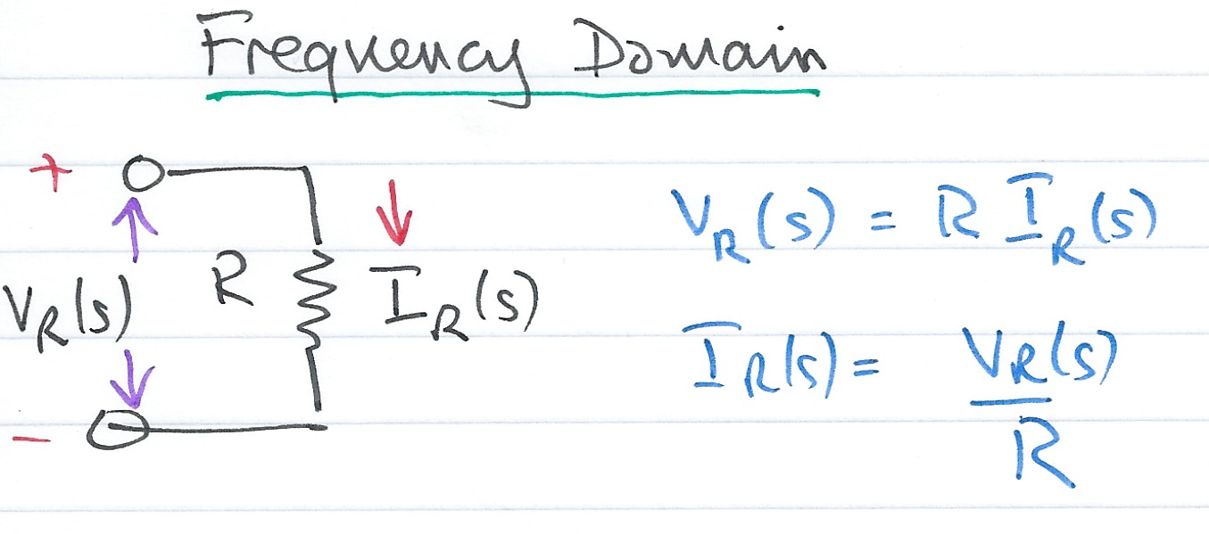
Fig. 51 Complex Frequency Domain Model of a Resistive Circuit#
Time Domain Model of an Inductive Network#
Consider Fig. 52
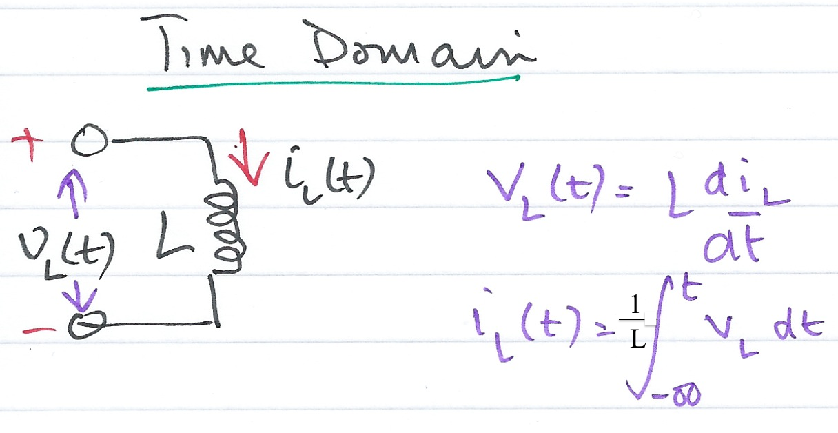
Fig. 52 Time Domain Model of an Inductive Network.#
In the time domain#
The voltage across the inductor \(i_L(t)\) is proportional to the rate of change of the current \(i_L(t)\) flowing through the inductor
eqvlt = v_L(t) == L*diff(i_L(t))
The current flowing through the inductor is inversely proportional to the integral of the voltage across the inductor which is easily confirmed by taking the integral of both sides of (22) and rewriting the equation to isolate \(i_L(t)\)
int(lhs(eqvlt)) == int(rhs(eqvlt));
eqilt = isolate(ans,i_L(t))
Rewritten nicely as
From these results, which of the following equations represent the Laplace transform of the current flowing through, and the voltage across, the inductor \(L\)?
-> Open poll Q2
Complex Frequency Domain Model of an Inductive Network#
Consider Fig. 53
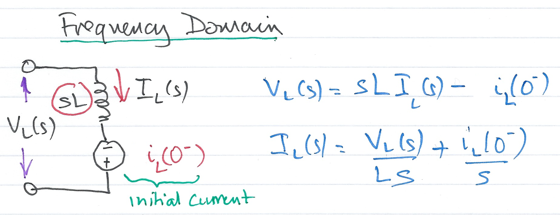
Fig. 53 Time Domain Model of a Resistive Network.#
In the complex frequency domain#
We take the Laplace transforms of (22) and (23) to obtain
Note
The current and voltage are transformed but so is the inductance. The complex frequency representation has used the derivative property for the voltage across the inductor and the integration properties for the current through the inductor. The use of the dervative and integration transforms has introduced a term that depends on the initial current flowing through the inductor. Therefore, the initial current would need to be considered in computing the actual voltage and current in the complex frequency domain.
Time Domain Model of a Capacitive Network#
Consider Fig. 54
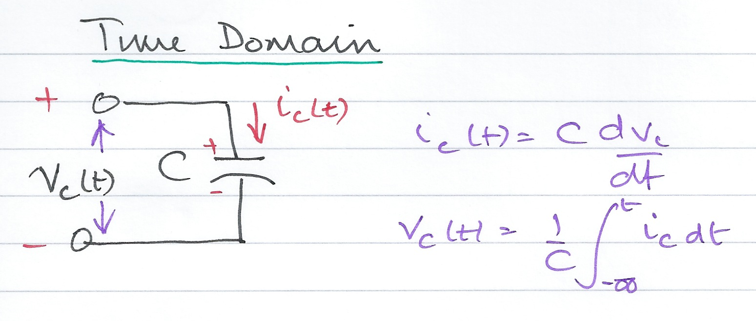
Fig. 54 Time Domain Model of a Capacitive Network.#
In the time domain#
The current flowing into the capacitor is proportional to the change in voltage across the capacitor
eqict = i_C(t) == C * diff(v_C(t))
The voltage across the capacitor is inversely proportional to the integral of the current flowing into the capacitor which is easily confirmed by taking the integral of both sides of (26) and rewriting the equation to isolate \(v_C(t)\)
int(lhs(eqict)) == int(rhs(eqict));
eqvct = isolate(ans,v_C(t))
Which can be rwritten nicely as
From the previous results, which of the following equations represent the Laplace transform of the current flowing into, and the voltage across, the capacitor \(C\)?
-> Open poll Q3
In the complex frequency domain#
We take the Laplace transforms of (26) and (27) to obtain
Note
The current and voltage are transformed but so is the capacitance. The complex frequency representation has used the derivative property for the voltage across the capacitor and the integration property for the current flowing into the capacitor. The use of the dervative and integration transforms has introduced a term that depends on the initial voltage (initial charge) across the capacitor. Therefore, the initial voltage would need to be considered in computing the actual voltage and current introduced by the capacitor in the complex frequency domain.
Complex Frequency Domain of a Capacitive Network#
Consider Fig. 55
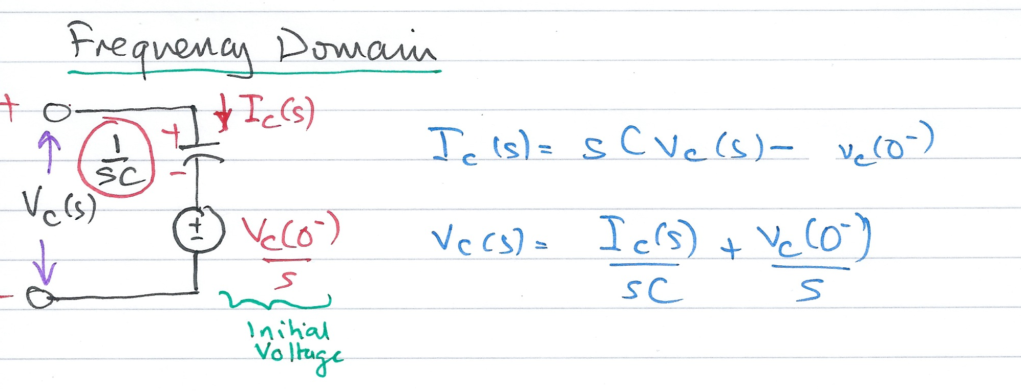
Fig. 55 Time Domain Model of a Capacitive Network.#
Exercises 12#
Do exercises 12.1 and 12.2 Now
Complex Impedance \(Z(s)\)#
By analogy with the resistance of a resistor \(R\), a component with complex impedance \(Z(s)\) satisfies Ohm’s law:
from which
Complex impedance of components#
For the resistance \(R\)\(\Omega\), inductance \(L\)H and capacitance \(C\)F, which of the following represent the complex impedance, \(Z(s) = V(s)/I(s)\) of the components?
-> Open Poll Q4
Consider the \(s\)-domain RLC series circuit shown in Fig. 56, where the initial conditions are assumed to be zero.
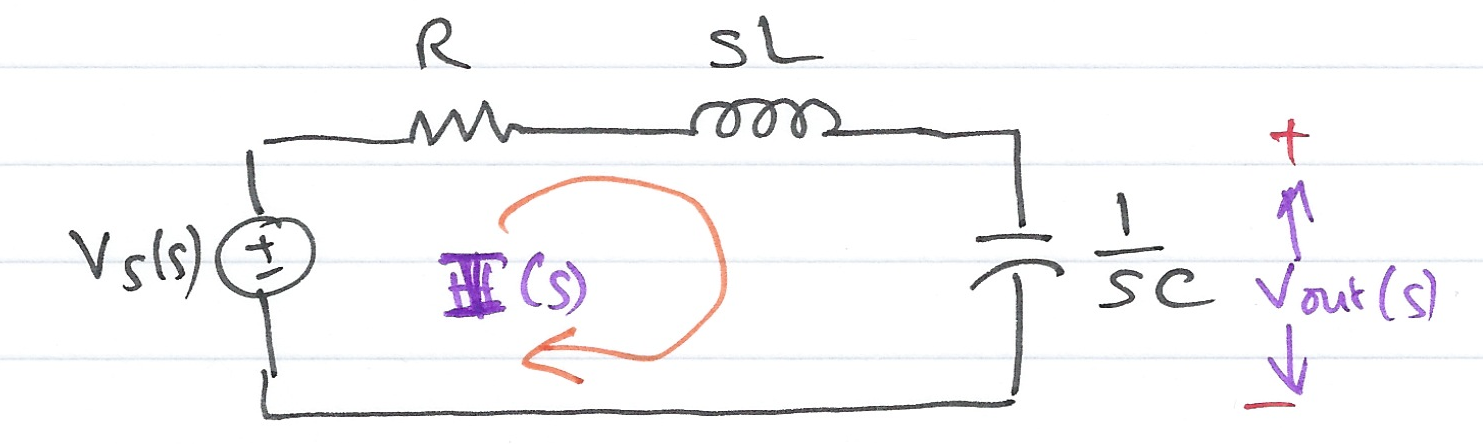
Fig. 56 RLC series circuit#
For this circuit, the sum
represents that total opposition to current flow.
Then,
and defining the ratio \(V_s(s)/I(s)\) as \(Z(s)\), we obtain
The \(s\)-domain current \(I(s)\) can be found from
where
Since \(s = \sigma + j\omega\) is a complex number, \(Z(s)\) is also complex and is known as the complex input impedance of this RLC series circuit.
Complex Admittance \(Y(s)\)#
By analogy with the admittance of a resistor \(G\), a component with complex admittance \(Y(s)\) satisfies Ohm’s law:
from which
Complex admittance of components#
For the resistance \(R\)\(\Omega\), inductance \(L\)H and capacitance \(C\)F, which of the following represent the complex admittance, \(Y(s) = I(s)/V(s)\) of the components?
For the resistor \(R\)Ω, inductor \(L\)H and capacitance \(C\)F, which of the following represent the complex admittance of the components?
-> Open Poll Q5
Consider the \(s\)-domain GLC parallel circuit shown in Fig. 57 where the initial conditions are zero.
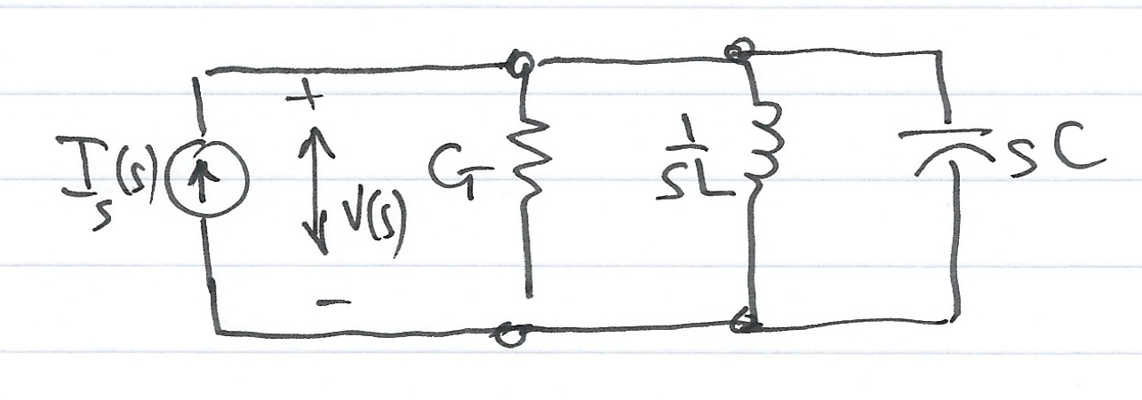
Fig. 57 A GLC parallel circuit#
For this circuit
Defining the ratio \(I_s(s)/V(s)\) as \(Y(s)\) we obtain
The \(s\)-domain voltage \(V(s)\) can be found from
where
\(Y(s)\) is complex and is known as the complex input admittance of this GLC parallel circuit.
Exercises 12#
We will work through these in class.
Exercise 12.1: RC circuit solved by KCL#
Note
This is based on Example 4.1 from [Karris, 2012].
Use the Laplace transform method and apply Kirchoff’s Current Law (KCL) to find the voltage \(v_c(t)\) across the capacitor for the circuit in Fig. 58 given that \(v_c(0^-) = 6\) V.
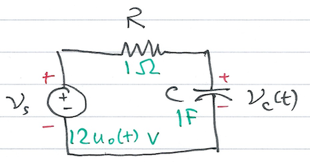
Fig. 58 Circuit for Example 12.1#
Exercise 12.2: RC circuit solved by KVL#
Note
This is based on Example 4.2 from [Karris, 2012].
Use the Laplace transform method and apply Kirchoff’s Voltage Law (KVL) to find the voltage \(v_c(t)\) across the capacitor for the circuit shown in fig:12.2 given that \(v_c(0^-) = 6\) V.
Fig. 59 Circuit for Example 12.2#
Exercise 12.3: A complex RLC circuit with initial conditions#
MATLAB Example
This is based on Example 4.3 in [Karris, 2012].
We will solve this example by hand in Examples class 4 and then review the solution in MATLAB lab 5.
In the circuit shown in Fig. 60, switch \(S_1\) closes at \(t=0\), while at the same time, switch \(S_2\) opens. Use the Laplace transform method to find \(v_{\mathrm{out}}(t)\) for \(t > 0\).
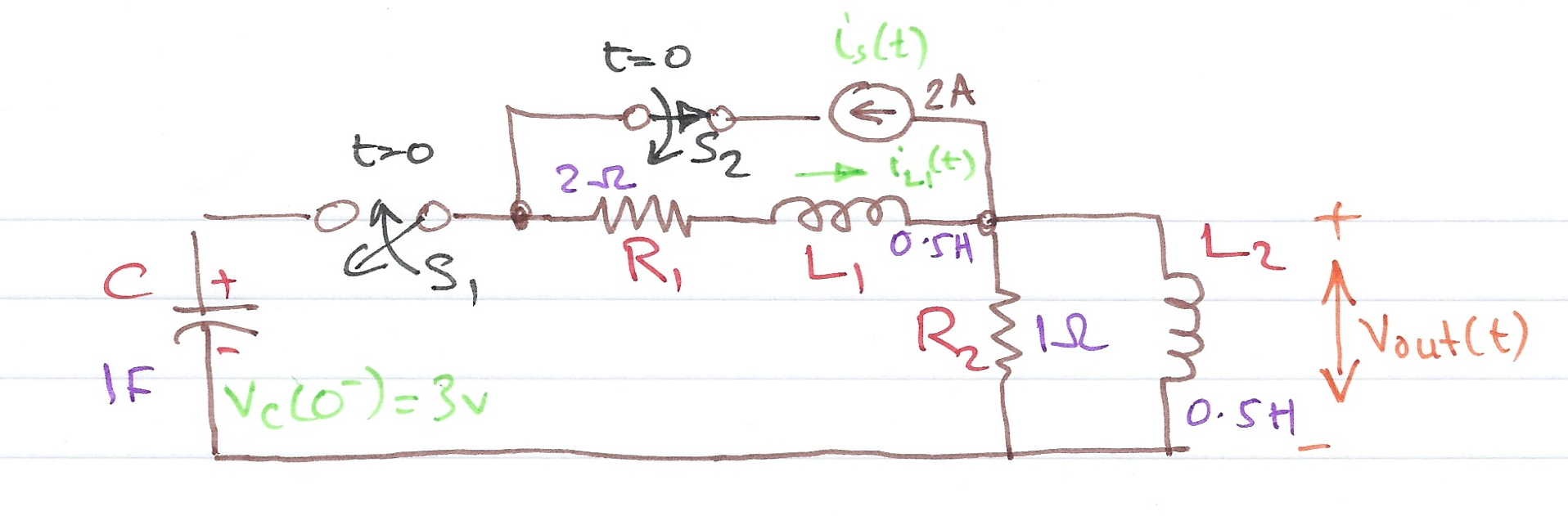
Fig. 60 Circuit for Example 12.3#
We can show how with the assistance of MATLAB (See solution12_3.mlx) that the solution is the inverse Laplace transform of
Which is $\(v_{\mathrm{out}}(t)=\left(1.36e^{-6.57t}+0.64e^{-0.715t}\cos 0.316t - 1.84e^{-0.715t}\sin 0.316t\right)u_0(t)\)$ (sol:12.3)
and we can plot the result (see 4. Complete solution in MATLAB)
open solution12_3
Worked Solution: Exercise 12.3: A complex RLC circuit with initial conditions#
File Pencast: example12_3.pdf - Download and open in Adobe Acrobat Reader.
The attached PDF gives the solution to Exercise 12.3: A complex RLC circuit with initial conditions by hand. It’s quite a complex, error-prone (as you can see by the crosssings out!) calculation that needs careful attention to detail. This in itself gives justification to my belief that you should use computers wherever possible.
Solution to Example 12.3#
We will use a combination of pen-and-paper and MATLAB to solve this.
1. Equivalent Circuit#
Draw equivalent circuit at \(t = 0\)
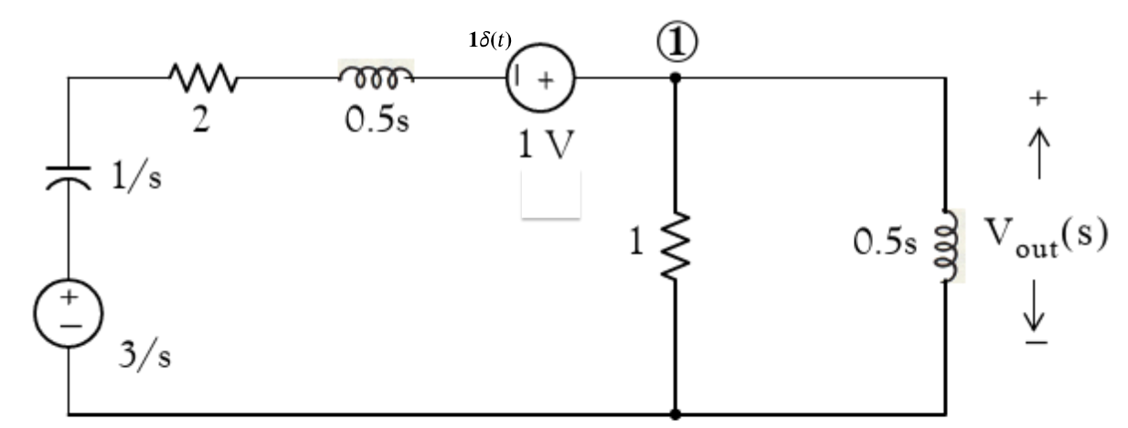
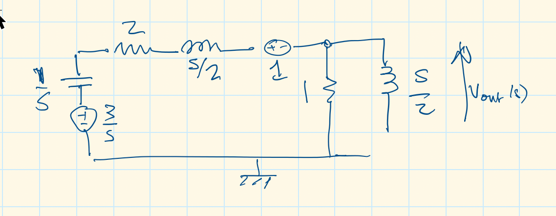
2. Transform model#
Convert to transforms
3. Determine equation#
Determine equation for \(V_{\rm out}(s)\).
syms s t vout Vout

eq45 = (Vout - 1 - 3/s)/(1/s + 2 + s/2) + Vout/1 + Vout/(s/2) == 0

Vout = solve(eq45, Vout)
4. Complete solution in MATLAB#
In the lecture we showed that after simplification for ex:12.3.1
We will use MATLAB to factorize the denominator \(D(s)\) of the equation into a linear and a quadratic factor.
Declare the denominator of \(V_{\mathrm{out}}(s)\) to be a polynomial in \(s\)
Ds = s^3 + 8*s^2 + 10*s + 4
Convert Ds to a MATLAB polynomial using sym2poly
d = sym2poly(Ds)
d = 1×4 double
     1     8    10     4
Find roots of \(D(s)\)
format long
p = roots(d)
p =
 -6.570750563722639 + 0.000000000000000i
 -0.714624718138679 + 0.313161257350729i
 -0.714624718138679 - 0.313161257350729i
Store real pole as p1
p1 = p(1)
Find quadratic form#
qs = expand((s - p(2))*(s - p(3)))
Simplify coefficients of s#
q = sym2poly(qs)
Complete the Square#
Left as an exercise for the reader
Compute the Residues#
Left as an exercise for the reader
Take inverse Laplace transform#
Numerator Ns
Ns = 2*s*(s + 3)
Denominator ‘Ds’ with quadratic factor
Ds = (s - p1)*qs
Vout = Ns/Ds
Exact solution
vout = ilaplace(Vout)
Approximate solution to 3 places of decimals
var = vpa(vout,3)
Plot result#
From equation sol:12.3
fplot(vout,[0,10]),...
    ylim([-0.5,2]),...
    grid,...
    title('Plot of Vout(t) for the circuit of Example 3'),...
    ylabel('Vout(t) V'),...
    xlabel('Time t s')
Alternative solution using transfer functions#
Vout = tf(2*conv([1, 0],[1, 3]),[1, 8, 10, 4])
impulse(Vout)
Exercise 12.4: RLC circuit#
Consider Fig. 56 and give an expression for \(V_c(s)\).
Exercise 12.5: Complex Impedance#
MATLAB Example
This is based on Example 4.4 from [Karris, 2012].
We will solve this examples by hand and then review the solution in MATLAB lab 5.
For the network shown in Fig. 61, all the complex impedance values are given in \(\Omega\) (ohms).
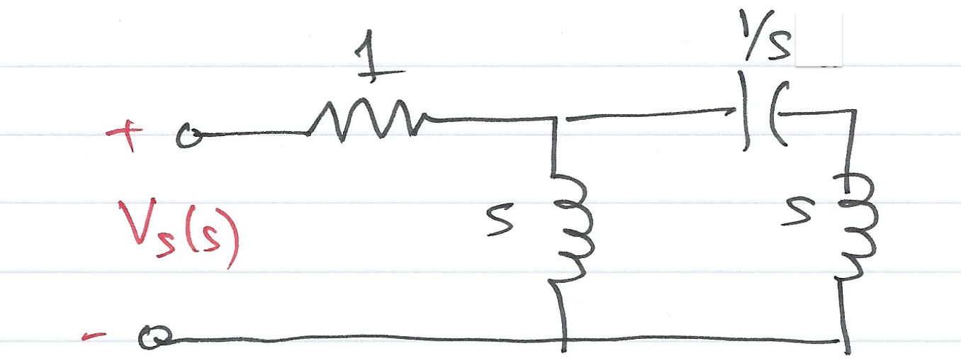
Fig. 61 Circuit for Example 12.5#
Find \(Z(s)\) using:
nodal analysis
by successive application of parallel and series combination of impedences
1. Solution by nodal analysis#
2. Solution by by successive application of parallel and series combination of impedences#
Solutions: Pencasts ex4_1.pdf and ex4_2.pdf – open in Adobe Acrobat.
Exercise 12.6: Complex admittance#
MATLAB Example
This is Example 4.5 from [Karris, 2012]
We will solve this examples by hand and then review the solution in MATLAB Lab 5.3.
Compute \(Z(s)\) and \(Y(s)\) for the circuit shown in Fig. 62. All impedence values are in \(\Omega\) (ohms). Verify your answers with MATLAB.
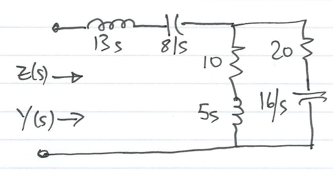
Fig. 62 Circuit for Example 12.6#
Answer 12.6#
Matlab verification: solution12_6.mlx
Example 12.6: Verification of Solution#
syms s;

z1 = 13*s + 8/s;
z2 = 5*s + 10;
z3 = 20 + 16/s;
z = z1 + z2 * z3 /(z2 + z3)
z10 = simplify(z)
pretty(z10)
Admittance#
y10 = 1/z10;
pretty(y10)
Exercise 12.7: Admittance and time response#
MATLAB Example
This is Exercise 4 from 4.7 Exercises from [Karris, 2012]
This example will be solved in MATLAB Lab 5.3.
For the s-domain circuit shown in Fig. 63
Compute the admittance \(Y(s) = I_1(s)/V_1(s)\)
Compute the time domain value of \(i_1(t)\) when \(v_1(t)=u_0(t)\) and all intial conditions are zero.
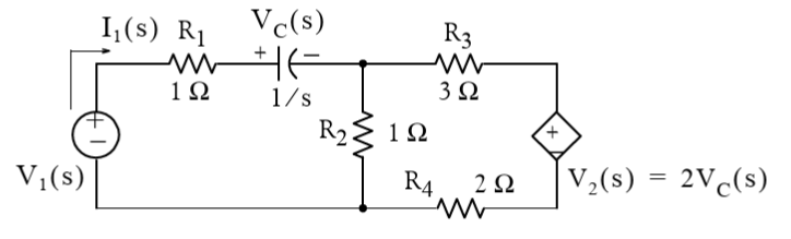
Fig. 63 Circuit for Example 12.7#
Lab Work#
In MATLAB Lab 5, we will explore the tools provided by MATLAB for solving circuit analysis problems.
Unit 4.5: Homework#
Complete any exercises that were not covered in the class or follow-up examples class. There are a number of related problems in Solved Problems 3.39—3.41 in [Hsu, 2020] and in section 4.7 Exercises in [Karris, 2012].
Supplementary problems 3.52 and following ([Hsu, 2020]) provide opportunities for extra practice.
Summary#
In this section we have looked at the application of the Laplace transform to circuit analysis.
Unit 4.5: Take Aways#
Circuit analysis can be performed using Laplace transforms by using the Laplace transform equivalents of the component impedence or admittance. In particular, for impedence, we use \(R\), \(sL\) and \(1/sC\); for admittance we use \(G = 1/R\), \(1/sL\), \(sC\). Once the circuit has been reduced to a rational polynomial in \(s\), the inverse laplace transform can be used to determine the time response of the circuit.
When dealing with components using their complex component equivalents, the usual circuit analysis rules, KVL, KCL, voltage-divider rule, etc, can all be used.
The complex impedence of a circuit is the resistance to current flow and is given by the general law \(V(s) = Z(s) I(s)\) from which the impendence is given by \(Z(s) = V(s)/I(s)\). Similarly, the complex admittance of a circuit is given by \(Y(s) = I(s)/V(s)\).
The complex admittance is the reciprocal of the complex impedence \(Y(s) = 1/Z(s)\).
Though not a consequence of the Laplace transform, it is worth noting that the use of impedence facilitates the analysis of circuits for which the components are commected in series; for circuits with parallel connection of components, the use of admittance facilitates the analsysis.
Next time#
We move on to consider
References#
Hwei P. Hsu. Schaums outlines signals and systems. McGraw-Hill, New York, NY, 2020. ISBN 9780071634724. Available as an eBook. URL: https://www.accessengineeringlibrary.com/content/book/9781260454246.
MATLAB Solutions#
For convenience, single script MATLAB solutions to the examples are provided and can be downloaded from the accompanying MATLAB folder in the GitHub repository.
Solution 12.3 [solution12_3.mlx]
Solution 12.6 [solution12_6.mlx]