Unit 4.6: Transfer Functions

Unit 4.6: Transfer Functions#

The preparatory reading for this section is 3.6 The System Function from [Hsu, 2020].

Follow along at cpjobling.github.io/eg-150-textbook/laplace_transform/6/transfer_functions

QR Code for this lecture

Agenda#

The Transfer Function
Characterization of LTI Systems
Transfer functions for LTI system described by Linear Constant-Coefficient Ordinary Differential Equations
Block diagrams for Systems Interconnection
Exercises 13: Transfer functions

The Transfer Function#

In Unit 3.1: Response of a Continuous-Time LTI System and the Convolution Integral we showed that the output $y (t)$ of a continuous-time LTI system equals the convolution of the input $x (t)$ with the impulse response $h (t)$ ; that is,

(31)#

y (t) = x (t) * h (t)

Applying the Convolution in the time domain property, we obtain

(32)#

Y (s) = X (s) H (s)

where $Y (s)$ , $X (s)$ , and $H (s)$ are the Laplace transforms of $y (t)$ , $x (t)$ , and $h (t)$ , respectively.

Equation (32) can be expressed as

(33)#

H (s) = \frac{Y (s)}{X (s)}

The laplace transform $H (s)$ of $h (t)$ is called the transfer function (or system function) of the system.

By (33), the transfer function $H (s)$ can also be defined as the ratio of the Laplace transforms of the output $y (t)$ and the input $x (t)$ .

The transfer function $H (s)$ completely characterizes the system because the impulse response $h (t)$ completely characterizes the system.

Fig. 64 illustrates the relationship of Equations and .

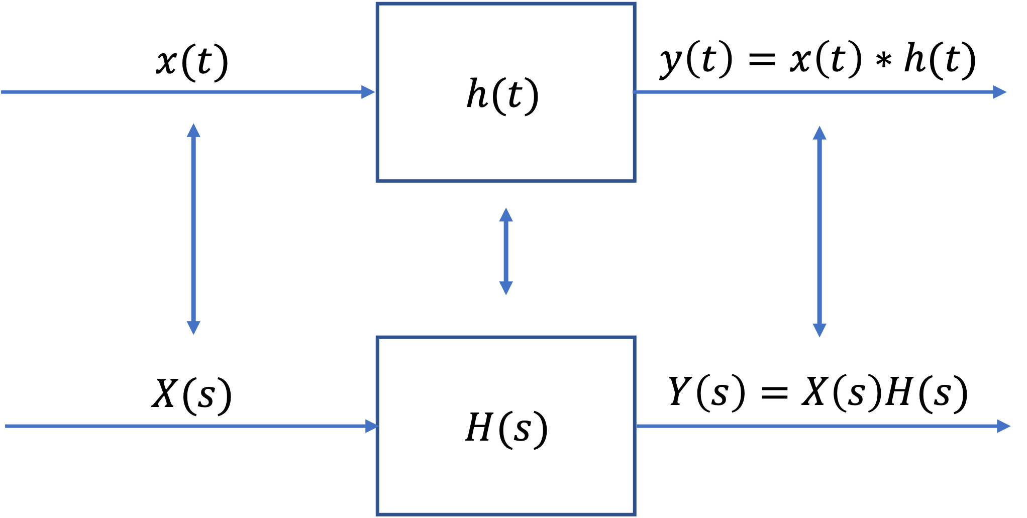
Impulse response and system function. — Fig. 64 Impulse response and system function#

Characterization of LTI Systems#

Note

This section is for reference only and is not examinable.

Many properties of continuous-time LTI systems can be closely associated with the characteristics of $H (s)$ in the $s$ -plane and in particular with the pole locations and the region of convergence (ROC).

Causality#

Fot a causal continuous-time LTI system, we have

h (t) = 0 t < 0

Since $h (t)$ is a right-sided signal, the corresponding requirement on $H (s)$ is that the ROC of $H (s)$ must be of the form

Re (s) > σ_{\max}

That is, the ROC is the region in the $s$ -plane to the right of all the system poles. Similarly, if the system is anticausal, then

h (t) = 0 t > 0

and $h (t)$ is left-sided. Thus, the ROC of $H (s)$ must be of the form

Re (s) < σ_{\max}

That is, the ROC is the region in the $s$ -plane to the left of all the system poles.

Stability#

In C. Stability we stated that a continuous-time LTI system is BIBO stable if and only if [Eq. (1)]

\int_{- \infty}^{\infty} | h (τ) | d τ < \infty

The corresponding requirement on $H (s)$ is that the ROC of $H (s)$ contains the $j ω$ axis (that is $s = j ω$ ). This is key result, proved in Prob. 3.26 in schaum, that is fundamental to systems and control theory.

Causal and stable systems#

If a system is both causal and stable then all the poles must be in the left-half of the $s$ -plane: that is they all have negative real parts because the ROC is of the form $Re (s) > σ_{\max}$ and since the $j ω$ axis is included in the ROC, we must have $σ_{\max} < 0$ .

The conditions for which the closed-loop poles in continuous-time LTI systems with feedback are stable is a key underlyting principle of the control theory to be studied in EG-243 Control Systems next year.

Transfer functions for LTI system described by Linear Constant-Coefficient Ordinary Differential Equations#

In Unit 3.3: Systems Described by Differential Equations we considered a continuous-time LTI systemfor which input $x (t)$ and output $y (t)$ satisfy the general linear constant-coefficient ordinary differential equation (LCCODE) of the form

(34)#

\sum_{k = 0}^{N} a_{k} \frac{d^{k}}{d t^{k}} y (t) = \sum_{k = 0}^{M} b_{k} \frac{d^{k}}{d t^{k}} x (t)

Applying the Laplace transform and using the Differentiation in the time domain of the Laplace transform, we obtain

\sum_{k = 0}^{N} a_{k} s^{k} Y (s) = \sum_{k = 0}^{M} b_{k} s^{k} X (s)

or

(35)#

Y (s) \sum_{k = 0}^{N} a_{k} s^{k} = X (s) \sum_{k = 0}^{M} b_{k} s^{k}

Thus,

(36)#

H (s) = \frac{Y (s)}{X (s)} = \frac{\sum_{k = 0}^{M} b_{k} s^{k}}{\sum_{k = 0}^{N} a_{k} s^{k}}

Expanding (36), $H (s)$ can be written in the more familiar form

(37)#

H (s) = \frac{Y (s)}{X (s)} = \frac{b_{M} s^{M} + b_{M - 1} s^{M - 1} + \dots + b_{1} s + b_{0}}{a_{N} s^{N} + b_{N - 1} s^{N - 1} + \dots + a_{1} s + a_{0}}

Hence, $H (s)$ is always a rational polynomial in $s$ .

Note the ROC of $H (s)$ is not specified by (36) but must be inferred with additional requirements on the system such as causality and stability.

Block diagrams for Systems Interconnection#

For two LTI systems (with $h_{1} (t)$ and $h_{2} (t)$ , respectively) in cascade (Fig. 65(a)), the overall impulse response is given

h (t) = h_{1} (t) * h_{2} (t)

Thus, the corresponding transfer functions are related by the product

(38)#

H (s) = H_{1} (s) H_{2} (s)

This relationship is illustrated in Fig. 65(b)

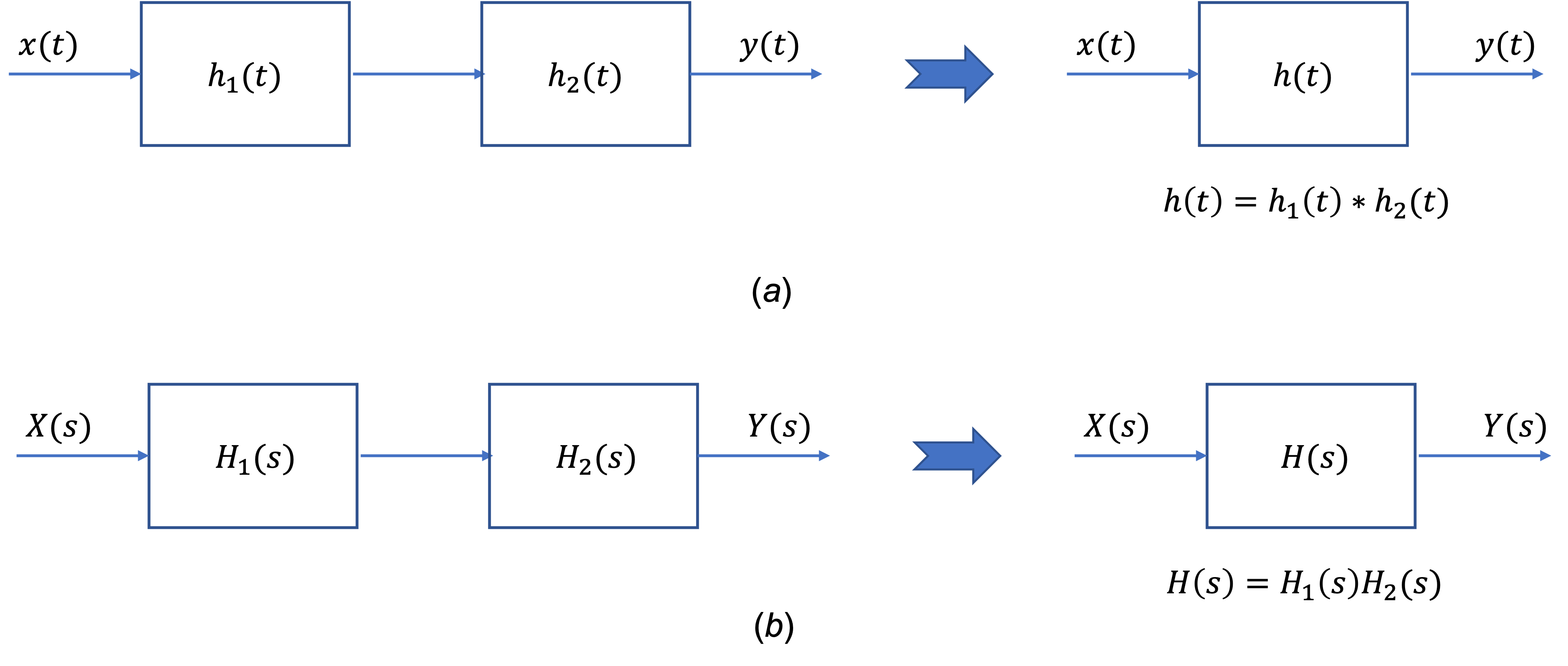
Two systems in cascade (a) Time-domain representation; (b) s-domain presentation. — Fig. 65 Two systems in cascade (a) Time-domain representation; (b) s-domain representation.#

Similarly, the impulse response of a parallel combination of two LTI systems (Fig. 66(a)) is given by

h (t) = h_{1} (t) + h_{2} (t)

Thus,

(39)#

H (s) = H_{1} (s) + H_{2} (s)

This relationship is illustrated in Fig. 66(b).

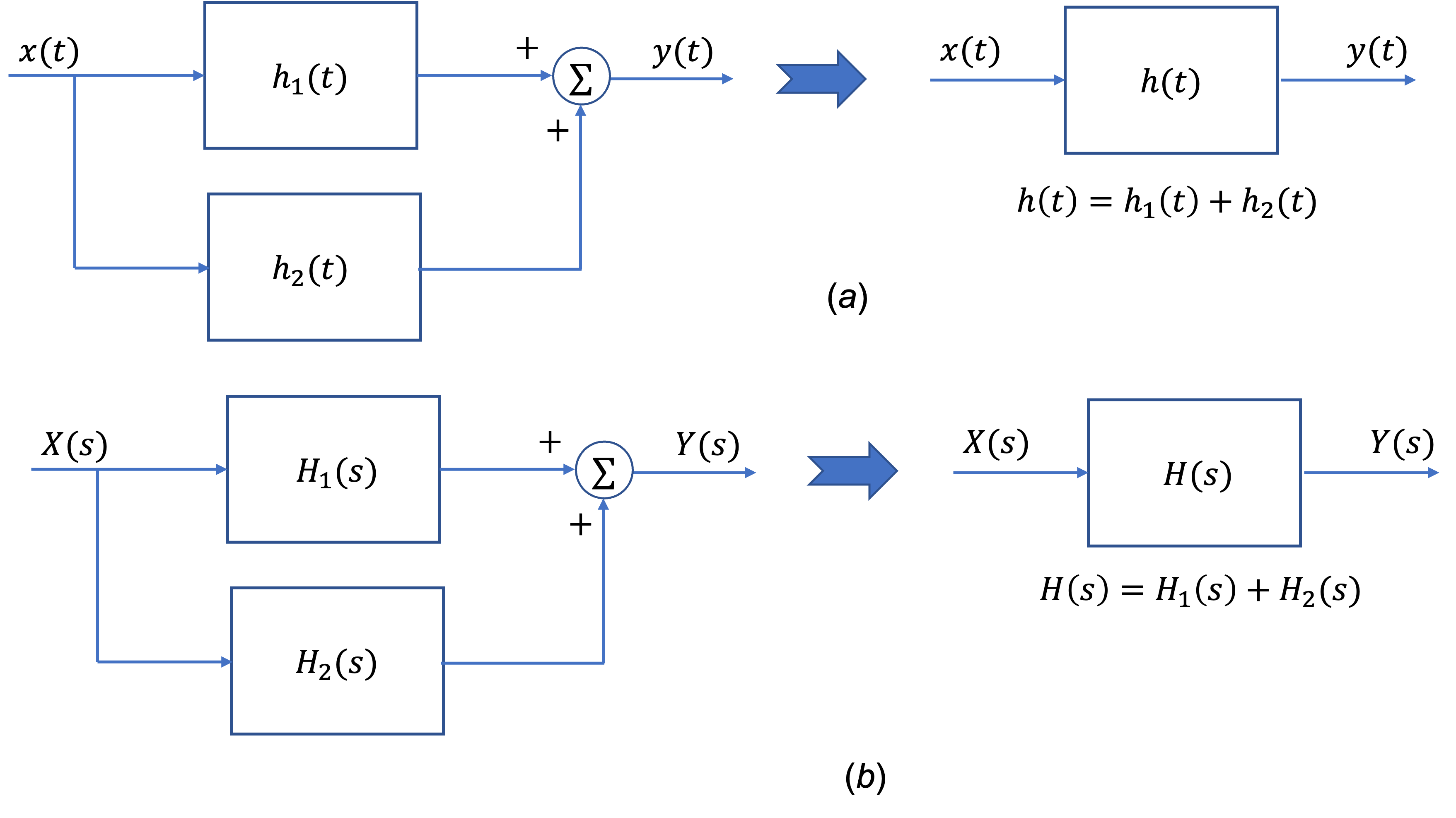
Fig. 66 Two systems in parallel. (a) Time-domain representation; (b) s-domain representation.#

Exercises 13: Transfer functions#

Exercise 13.1: RC circuit#

Find the transfer function $H (s)$ and the impulse reponse $h (t)$ of the RC circuit in Fig. 30 (Exercise 4.1: RC Circuit).

For the answer, refer to the lecture recording or see solved problem 3.23 in in [Hsu, 2020].

Exercise 13.2: Step response#

Use the Laplace transform to redo Exercise 5.5.

For the answer, refer to the lecture recording or see solved problem 3.24 in in [Hsu, 2020].

Exercise 13.3: Impulse response from step response#

The output $y (t)$ of a continuous-time LTI system is found to be $2 e^{- 3 t} u_{0} (t)$ when the input $x (t)$ is $u_{0} (t)$ .

a). Find the impulse response $h (t)$ of the system.

b). Find the output $y (t)$ when the input is $e^{- t} u_{0} (t)$ .

For the answer, refer to the lecture recording or see solved problem 3.25 in in [Hsu, 2020].

Exercise 13.4: Convolution#

Use the Laplace transform to redo Exercise 6.6.

For the answer, refer to the lecture recording or see solved problem 3.27 in in [Hsu, 2020].

Exercise 13.5: Differential equation 1#

Use the Laplace transform to redo Exercise 8.6.

For the answer, refer to the lecture recording or see solved problem 3.28 in in [Hsu, 2020].

Exercise 13.6: Differential equation 2#

Use the Laplace transform to redo Exercise 8.8.

For the answer, refer to the lecture recording or see solved problem 3.29 in in [Hsu, 2020].

Exercise 13.7: Differential equation 3#

Consider a continuous-time LTI system for which the input $x (t)$ and output $y (t)$ are related by

(40)#

\frac{d^{2} y (t)}{d t^{2}} + \frac{d y (t)}{d t} - 2 y (t) = x (t)

a) Find the transfer function $H (s)$

b) Find the impulse response $h (t)$

For the answer, refer to the lecture recording or see solved problem 3.30 in in [Hsu, 2020].

Exercise 13.8: Feedback#

The feedback interconnection of two causal subsytems with transfer functions $F (s)$ and $G (s)$ is shown in Fig. 67. Find the overall system function $H (s)$ for this feedback system.

For the answer, refer to the lecture recording or see solved problem 3.31 in in [Hsu, 2020].

Unit 4.6: Homework#

Attempt any of the questions in Exercises 12 of these course notes that have not been covered in the examples class.

The solutions for Unit 4.6 are in Section 3.8 Solved Problems [Hsu, 2020] starting at 3.23. (The actual numbers are listed with the examples above.)

We will do some problems from these sets in Examples Class 4.

Supplementary Problems#

Supplementary problems 3.52-3.55 in [Hsu, 2020] are related to the content covered in this unit.

Summary#

In this unit we have presented the idea of a transfer function (or system function) that allows us to represent the impulse response $h (t)$ by the Laplace transform $H (s)$ . We also looked at the characteristics of the Laplace transform, transform functions for LCCODEs and series and parallel combination of transfer functions.

The Transfer Function
Characterization of LTI Systems
Transfer functions for LTI system described by Linear Constant-Coefficient Ordinary Differential Equations
Block diagrams for Systems Interconnection
Exercises 13: Transfer functions

Unit 4.6: Take Aways#

My main message to you is that, as an engineer faced with a LCCODE to solve, you should use Laplace transforms!

Transfer function#

The summary of the time-domain and s-domain transforms are illustrated in Fig. 64. The key result is $Y (s) = H (s) X (s)$ which simplifies the computation of the system response $y (t) = h (t) * x (t)$ which has to be done using time-convolution.

If we know $Y (s)$ and $X (s)$ we can determine $H (s)$ using

H (s) = \frac{Y (s)}{X (s)}

and $h (t) = L^{- 1} {H (s)}$

Characterization of LTI Systems#

For continuous-time LTI systems the causality and stabilty of a system is guaranteed if all the poles of the transfer function are in the left-half of the $s$ -plane and the $j ω$ axis is included in the region of convergence. That is, if the poles of the system $H (s)$ , $s_{k}$ have real part $- σ_{k}$ , the system will be causal and stable if $σ_{k} < 0$ for all $k$ .

Laplace transforms of LCCODEs#

The linear constant coefficient ordinary differential equation (LLCODE) of a system involving input signal $x (t)$ and output signal $y (t)$ is given in (34). When we take Laplace transforms of this differential equation, ignoring initial conditions, we get the polynomial equation (35) from which we can determine the transfer function:

H (s) = \frac{Y (s)}{X (s)} = \frac{b_{M} s^{M} + b_{M - 1} s^{M - 1} + \dots + b_{1} s + b_{0}}{a_{N} s^{N} + b_{N - 1} s^{N - 1} + \dots + a_{1} s + a_{0}}

This is a rational polynomial in $s$ and it can be solved for any input $x (t)$ that has a Laplace transform $X (s)$ by forming

Y (s) = H (s) X (s)

and taking inverse Laplace transforms using the Partial Fraction Expansion method discussed in Unit 4.5: Using Laplace Transforms for Circuit Analysis.

Several examples are given in Exercises 12 in which the problems given in examples8 of unit3.3 are redone as Laplace transform problems.

Block diagrams#

Complex systems can be broken down into subsystems which may be represented by block diagrams which have either series or parallel connections (see Fig. 65 and Fig. 66 and feedback (See Exercise 13.8: Feedback)

Still to come#

We will use transfer functions to solve circuit problems in Unit 4.7: Transfer Functions for Circuit Analysis and conclude our study of Laplace transforms in Unit 4.8: Computer-Aided Systems Analysis and Simulation with a look at the use of Transfer functions in the MATLAB control systems toolbox and the simulation tool Simulink. We will also look at some of the problems you have studied in EG-152 Analogue Design hopefully confirming some of the results you have observed in the lab.

In EG-247 Digital Signal Processing we will start from the knowledge gained in Unit 4 developing transform ideas further via the Fourier Transform, Z-Transform and the design of systems for signal processing. In EG-243 Control Systems you will model feedback control signals using block diagrams and transfer functions. You will also study how knowledge of poles and zeros can be exploited in the design of systems with stable responses.

Next time#

We move on to consider

Unit 4.7: Transfer Functions for Circuit Analysis

References#

[Hsu20] (1,2,3,4,5,6,7,8,9,10,11)

Hwei P. Hsu. Schaums outlines signals and systems. McGraw-Hill, New York, NY, 2020. ISBN 9780071634724. Available as an eBook. URL: https://www.accessengineeringlibrary.com/content/book/9781260454246.

Unit 4.6: Transfer Functions

Contents

Unit 4.6: Transfer Functions#

Agenda#

The Transfer Function#

Characterization of LTI Systems#

Causality#

Stability#

Causal and stable systems#

Transfer functions for LTI system described by Linear Constant-Coefficient Ordinary Differential Equations#

Block diagrams for Systems Interconnection#

Exercises 13: Transfer functions#

Exercise 13.1: RC circuit#

Exercise 13.2: Step response#

Exercise 13.3: Impulse response from step response#

Exercise 13.4: Convolution#

Exercise 13.5: Differential equation 1#

Exercise 13.6: Differential equation 2#

Exercise 13.7: Differential equation 3#

Exercise 13.8: Feedback#

Unit 4.6: Homework#

Supplementary Problems#

Summary#

Unit 4.6: Take Aways#

Transfer function#

Characterization of LTI Systems#

Laplace transforms of LCCODEs#

Block diagrams#

Still to come#

Next time#

References#