Unit 4.3 Properties of the Laplace Transform#
The preparatory reading for this section is Chapter 2.3 of [Karris, 2012] and Chapter 3.3 of [Hsu, 2020].
Follow along at cpjobling.github.io/eg-150-textbook/laplace_transform/3/laplace_properties

Agenda#
Some Selected Properties of the Laplace transform#
Basic properties of the Laplace transform are presented in the following. Verification of these properties is given in Worked Problems 3.8 to 3.16 in [Hsu, 2020] and in Section 2.2 in [Karris, 2012].
We will verify some of the properties in MATLAB Lab 4, but will not examine them further in this course.
You will, however, be expected to use Tables of Properties, such as that given in Table of Laplace Transform Properties below, to solve problems.
Linearity#
Time shift#
Frequency shift#
Scaling#
Differentiation in the time domain#
This property facilitates the solution of differential equations
The differentiation property can be extended to higher-orders as follows
and in general
Differentiation in the complex frequency domain#
and in general
Integration in the time domain#
This property is important because it provides a way to model the solution of a differential equation using op-amp integrators in so-called Analogue Computers and is now the basis for numerical integration systems like Simulink.
Integration in the complex frequency domain#
Providing that
exists
Time periodicity property#
If \(f(t)\) is a periodic function with period \(T\) such that \(f(t) = f(t+nT)\) for \(n=1,2,3,\ldots\) then
Initial value theorem#
Final value theorem#
Convolution in the time domain#
This is another important result as it allows us to compute the response of a system by simply multiplying the Laplace transforms of the system and the signal and then inverse Laplace transforming the result.
This is usually much simpler than computing the convolution integral in the time domain – an operation we we met in C. Convolution Integral.
Convolution in the complex frequency domain#
Multiplying two signals together in the time domain is the same as performing convolution in the complex frequency domain.
Convolution in the complex frequency domain is nasty – multiplication in the time domain is relatively painless.
Table of Laplace Transform Properties#
No. |
Name |
Time Domain \(f(t)\) |
Complex Frequency Domain \(F(s)\) |
|---|---|---|---|
1. |
Linearity |
\(a_1f_1(t)+a_2f_2(t)+\cdots+a_nf_n(t)\) |
\(a_1F_1(s)+a_2F_2(s)+\cdots+a_nF_n(s)\) |
2. |
Time shifting |
\(\displaystyle{f(t-a)}u_0(t-a)\) |
\(\displaystyle{e^{-a s}F(s)}\) |
3. |
Frequency shifting |
\(\displaystyle{e^{-as}f(t)}\) |
\(\displaystyle{F(s+a)}\) |
4. |
Time scaling |
\(f(a t)\) |
\(\displaystyle{\frac{1}{a}F\left(\frac{s}{a}\right)}\) |
5. |
Time differentiation |
\(\displaystyle{\frac{d}{dt}\,f(t)}\) |
\(\displaystyle{F(s)-f(0^-)}\) |
7. |
Frequency differentiation |
\(\displaystyle{tf(t)}\) |
\(\displaystyle{-\frac{d}{ds}F(s)}\) |
8. |
Time integration |
\(\displaystyle{\int_{-\infty}^{t}f(\tau)d\tau}\) |
\(\displaystyle{\frac{F(s)}{s}+ \frac{F(0^-)}{s}}\) |
9. |
Frequency integration |
\(\displaystyle{\frac{f(t)}{t}}\) |
\(\displaystyle{\int_s^\infty F(s)\,ds}\) |
10. |
Time Periodicity |
\(\displaystyle{f(t + nT)}\) |
\(\displaystyle{\frac{\int_0^T f(t)e^{-st}\,dt}{1 - e^{-sT}}}\) |
11. |
Initial value theorem |
\(\displaystyle{\lim_{t\rightarrow 0} f(t)}\) |
\(\displaystyle{\lim_{s\rightarrow \infty}sF(s) = f(0^-)}\) |
12. |
Final value theorem |
\(\displaystyle{\lim_{t\rightarrow \infty} f(t)}\) |
\(\displaystyle{\lim_{s\rightarrow 0}sF(s) = f(\infty)}\) |
13. |
Time convolution |
\(\displaystyle{f_1(t)*f_2(t)}\) |
\(\displaystyle{F_1(js) F_2(s)}\) |
14. |
Frequency convolution |
\(\displaystyle{f_1(t)f_2(t)}\) |
\(\displaystyle{\frac{1}{j2\pi}F_1(s)*F_2(s)}\) |
See also: Wikibooks: Engineering_Tables/Laplace_Transform_Properties and Laplace Transform—WolframMathworld for more complete references.
Exercises 10: Laplace transforms of common waveforms#
We will work through a few of the following on the board in class
Exercise 10.1: Pulse#
Use the tables of Laplace transforms and properties as appropriate to compute the Laplace transform of the pulse shown in Fig. 45.
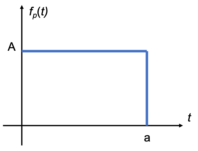
Fig. 45 A rectangular pulse.#
For full solution see Example 2.4.1 in Karris.
Exercise 10.2: Line segment#
Use the tables of Laplace transforms and properties as appropriate to compute the Laplace transform of the line segment shown in Fig. 46.
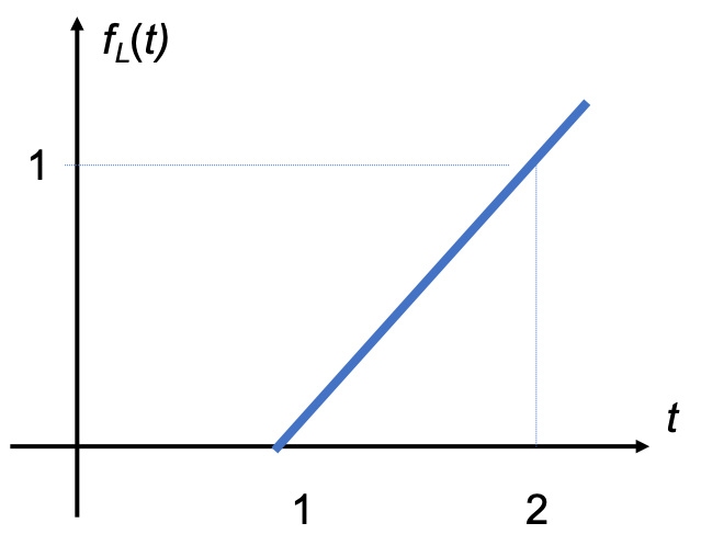
Fig. 46 A line segment.#
For full solution see Example 2.4.2 in Karris.
Exercise 10.3: Triangular Pulse#
Use the tables of Laplace transforms and properties as appropriate to compute the Laplace transform of the triangular pulse shown in Fig. 47.
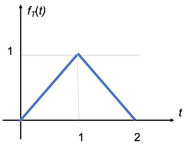
Fig. 47 A triangular pulse.#
For full solution see Example 2.4.3 in Karris.
Exercise 10.4: Square Wave#
Use the tables of Laplace transforms and properties as appropriate to compute the Laplace transform of the of the periodic function shown in Fig. 48.
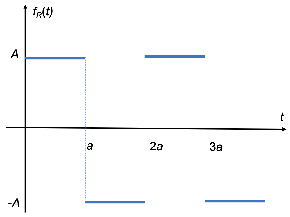
Fig. 48 A square wave.#
For full solution see Example 2.4.4 in Karris.
Exercise 10.5: Half-rectified Sinewave#
Use the tables of Laplace transforms and properties as appropriate to compute the Laplace transform of the half-rectified sine wave shown in Fig. 49.
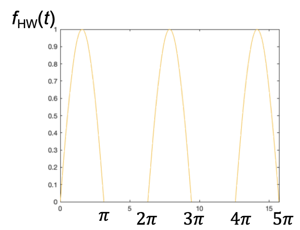
Fig. 49 Half-rectified sine wave.#
For full solution see Example 2.4.5 in Karris.
Unit 4.3: Homework#
Attempt at least one of the end-of-chapter exercises from each question 1-7 of Section 2.7 of [Karris, 2012]. Don’t look at the answers until you have attempted the problems.
If we have time, I will work through one or two of these in class.
Summary#
In this section we have presented some of the most useful and commonly used properties of the Laplace transform, provided a table of Laplace Transform properties, and given examples of how properties and transform tables can be used to determine the Laplace transform of some useful aperiodic and periodic signals.
Unit 4.3: Take Aways#
There are a number of useful properties of the Laplace transform that we can use to simplify more complex problems in signals and systems, for example to find the laplace transforms of more complex signals than those studied in Unit 4.2: Laplace Transform of Some Common Signals. In particular we found that the time delay property \(f(t-a) \Leftrightarrow e^{-as}F(s)\) and the linearity property \(c_1f_1(t) + c_2f_2(t) + \ldots + c_nf_n(t) \Leftrightarrow c_1F_1(s) + c_2F_2(s) + \ldots + c_nF_n(s)\) are particularly useful.
If you have a periodic signal \(x(t) = x(t + nT)\), you must use the periodicity property
to compute its Laplace transform.
Still to come#
The use of the derivative property and integration property will be useful when defining the complex frequency equavalent of the time domain models used to define electrical circuit components. We study these in detail in Unit 4.5: Using Laplace Transforms for Circuit Analysis. The use of the derivative property will be used to determine the complete solution of continuous-time LTI systems defined by differential equations in Unit 4.6: Transfer Functions. More practice in the use of Laplace transforms will be covered in Lab 4.
Next time#
We move on to consider
References#
Hwei P. Hsu. Schaums outlines signals and systems. McGraw-Hill, New York, NY, 2020. ISBN 9780071634724. Available as an eBook. URL: https://www.accessengineeringlibrary.com/content/book/9781260454246.
Steven T. Karris. Signals and systems with MATLAB computing and Simulink modeling. Orchard Publishing, Fremont, CA., 2012. ISBN 9781934404232. Library call number: TK5102.9 K37 2012. URL: https://ebookcentral.proquest.com/lib/swansea-ebooks/reader.action?docID=3384197.
Answers to Exercises 10#
Exercise 10.3: Triangular Pulse
Exercise 10.5: Half-rectified Sinewave