Unit 5.1: Qualitative Properties of Signals and Transfer functions

Unit 5.1: Qualitative Properties of Signals and Transfer functions#

Follow along at cpjobling.github.io/eg-150-textbook/poles_and_zeros/qualitative_properties

QR Code for this lecture

Acknowledgements#

The notes for this section have been adapted from Qualitative properties of signals & Laplace transforms [Boyd, 1993] and was also partly influenced by the MATLAB LiveScript PoleZeroAnalysis.mlx from the MathWorks curriculum module Transfer Function Analysis of Dynamic Systems [Allie, 2024].

format compact
cd matlab

Agenda#

Inverse Laplace transform of a rational F(s)
Qualitative properties of terms
Quantitative properties of terms
Complex poles: Damping ratio \zeta and quality factor Q
Dominant Poles
Stability of autonomous LCCODEs
Initial value theorem
Final value theorem

Inverse Laplace transform of a rational $F (s)$ #

Suppose $F (s) = N (s) / D (s)$ is rational and strictly proper[1] with $L^{- 1} {F (s)} = f (t)$ each term in the partial fraction expansion of $F (s)$ gives a term in $f (t)$ :

For a single pole at $s = λ$ [2],

(46)#

L^{- 1} {\frac{1}{s - λ}} = e^{λ t}

For a pole at $s = λ$ of multiplicity $k$ ,

(47)#

L^{- 1} {\frac{1}{{(s - λ)}^{k}}} = \frac{1}{(k - 1)!} t^{k - 1} e^{λ t}

The poles of $F (s)$ determine the types of terms that appear in $f (t)$ .

The zeros (or residues) of $F (s)$ determine the coeficients multiplying each term, or the amplitude and phase of oscillitory terms.

Qualitative properties of terms#

Real poles#

Real, positive poles correspond to growing exponential terms.

Real, negative poles correspond to decaying exponential terms.

A pole at $s = 0$ corresponds to a constant (DC) term.

Complex poles#

Complex pole pairs with positive real part correspond to exponentially growing sinusoidal terms.

Complex pole pairs with negative real part correspond to exponentially decaying sinusoidal terms.

Imaginary poles#

Pure imaginary pole pairs correspond to sinusoidal terms.

Repeated poles#

Repeated poles yield the same types of terms, multiplied by powers of $t$ .

Quantitative properties of terms#

The pole $λ_{1} = σ + j ω$ and its conjugate pair $\bar{λ} = \overset{―}{(σ + j ω)} = σ - j ω$ [^pz:note3]

Re λ = σ, Im λ = ω

will yield a time domain term

(48)#

a e^{σ t} \cos (ω t + ϕ) .

The real part of the pole gives the growth rate (if positive) or decay rate (if negative) of the corresponding term in $f (t)$ .

The imaginary part gives the oscillation frequency.

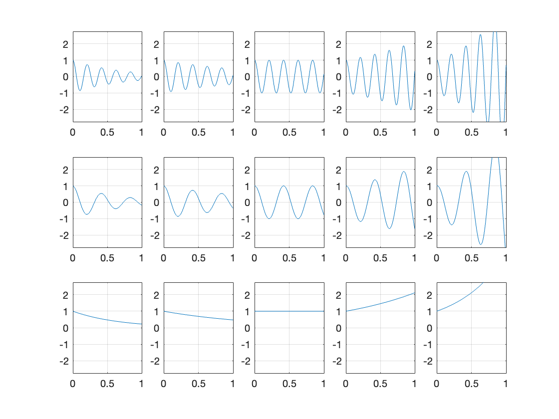
Example 1#

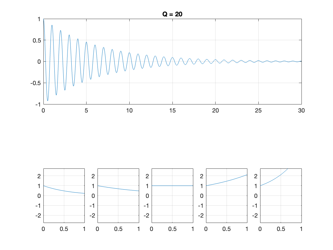
Quantifying the response for $f (t) = e^{σ t} \cos (ω t)$ : rows $ω = 30, 15, 0$ ; columns: $σ = - 1.5, - 0.75, 0, 0.75, 1.5$

example1

../_images/f16583fd88982a6b9351d272f961aecad70c642f8138c2ee96f57808d1ce49d0.png

The MATLAB code to reproduce this figure is given in example1.mlx

open example1

Qualitative analysis from the pole-zero map#

By plotting the poles and zeros on the $s$ -plane we can say quite a lot about the expected response. These ideas are summarized in Fig. 74.

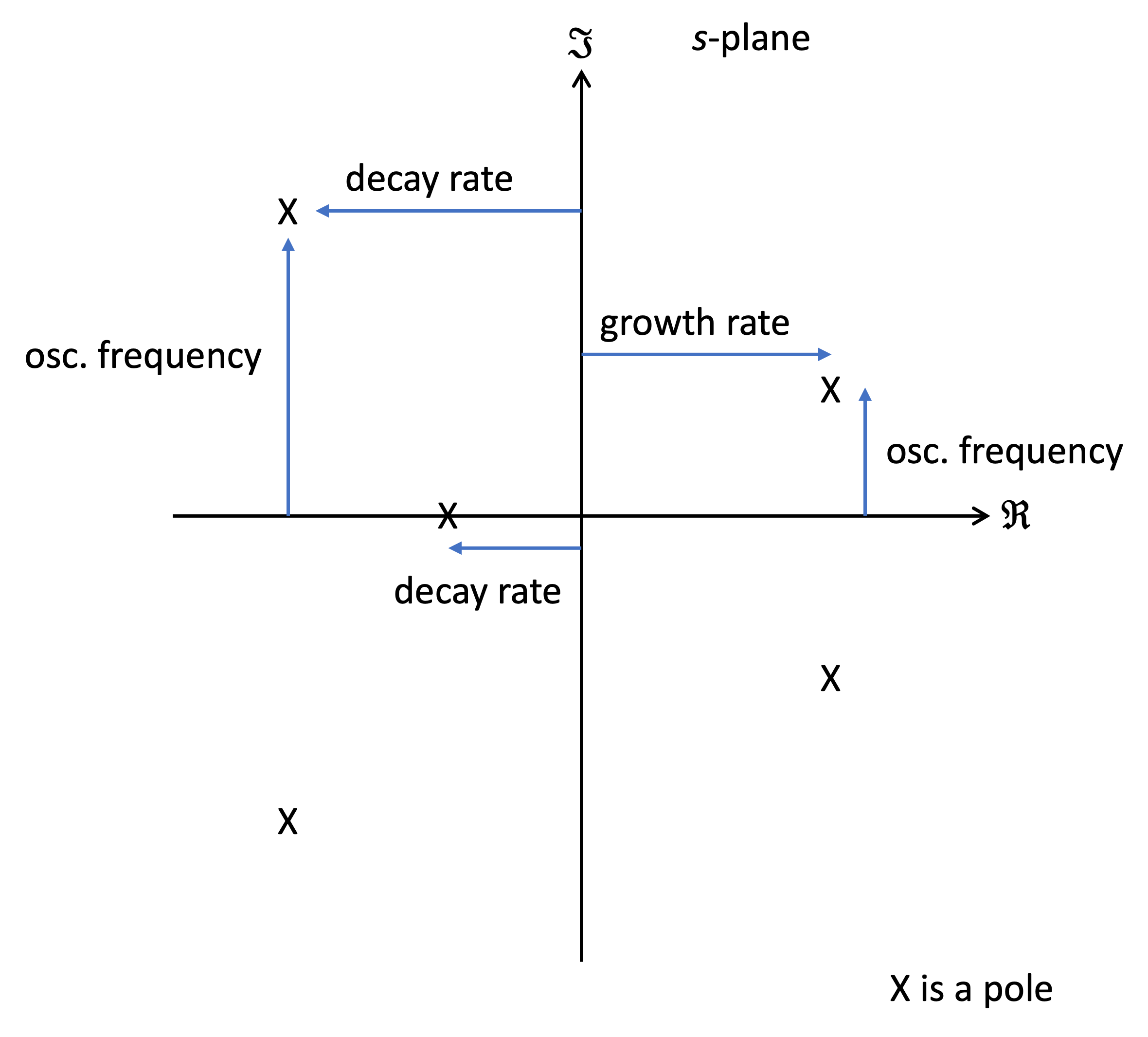
A figure illustrating the quantitive properties of terms f(t) resulting from the poles of F(s). — Fig. 74 Illustrating the quantitive properties of the terms $f (t)$ resulting from the poles of $F (s)$ #

Complex poles: Damping ratio $ζ$ and quality factor $Q$ #

For a pole at $s = λ = σ + j ω$ (hence also at $\bar{λ}$ ) with $σ < 0$ :

F (s) = \frac{r}{s + σ + j ω} + \frac{\bar{r}}{s + σ - j ω}

F (s) = \frac{2 Re (r) s - 2 Re (r λ)}{s^{2} + 2 σ s + (σ^{2} + ω^{2})}

which resolves to

f (t) = a e^{- σ t} \cos (ω t + ϕ)

There are two measures of the decay rate per cycle of oscillation:

damping ratio

(49)#

ζ = \frac{- σ}{\sqrt{σ^{2} + ω^{2}}}

quality factor

(50)#

Q = \frac{1}{2} \sqrt{\frac{σ^{2} + ω^{2}}{σ^{2}}} = \frac{1}{2 ζ}

The damping ratio (or $Q$ ) is related to the $a n g l e$ of the pole in the complex plane as shown in Fig. 75:

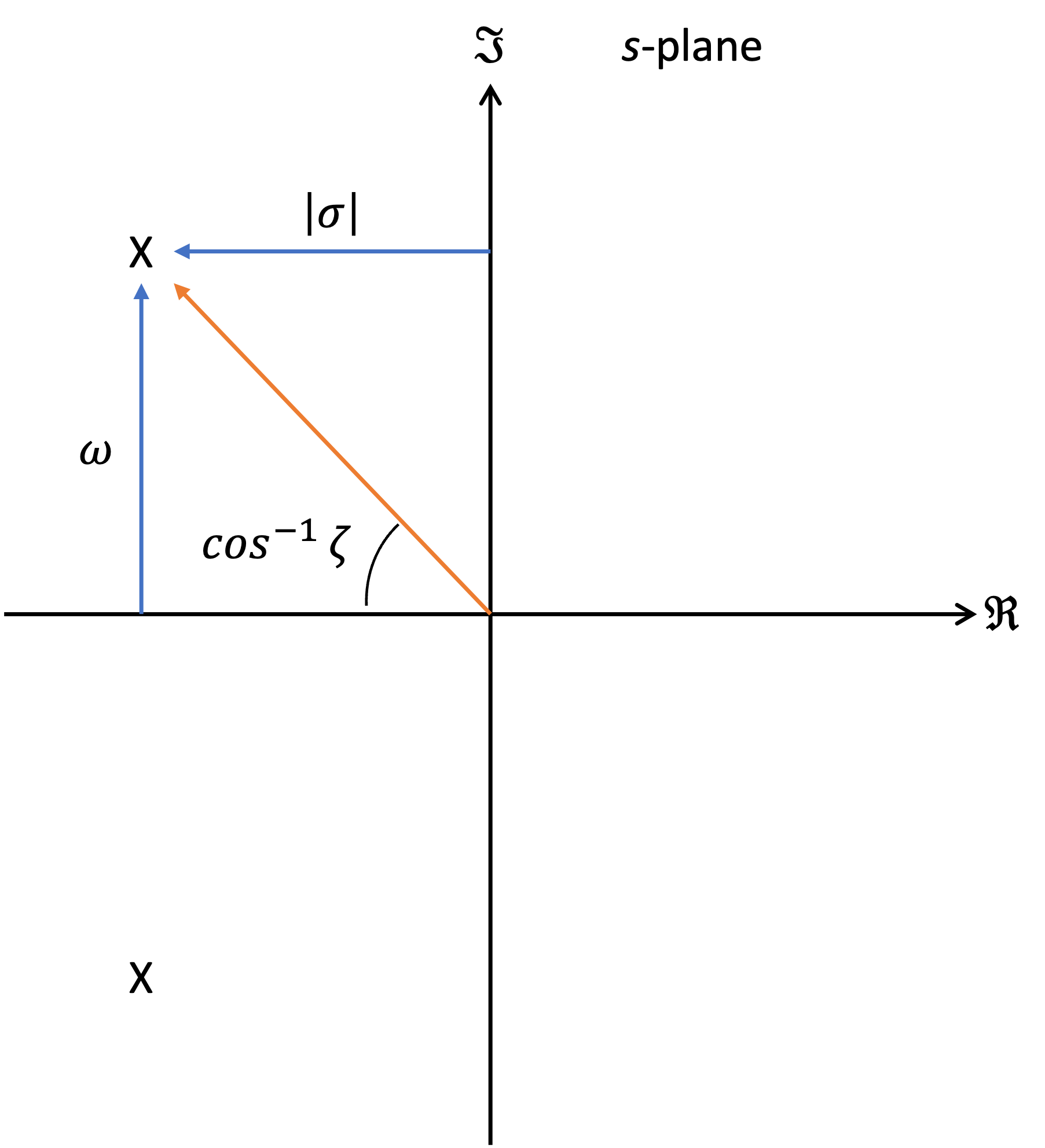
Fig. 75 The damping ratio is related the the angle of the pole in the complex plane#

There is another concept in this diagram that we will refer to later.

If we consider the polar form of the pole illustrated by the red line in Fig. 76

λ_{1, 2} = - σ \pm j ω = - ω_{n} e^{\pm j θ}

where $θ = \cos^{- 1} ζ$ and $ω_{n} = \sqrt{σ^{2} + ω^{2}}$ is called the natural frequency.

We will say more about the damping ratio $ζ$ and natural frequency $ω_{n}$ in Unit 5.2: More on the Qualitative and Quantitative Response of First- and Second-Order Poles.

The oscillation is

underdamped: $ζ < 1$ ( $Q > 1 / 2$ )

critically damped: $ζ = 1$ ( $Q = 1 / 2$ )

Example 2: parallel RLC circuit#

Consider the parallel RLC citcuit shown in Fig. 76.

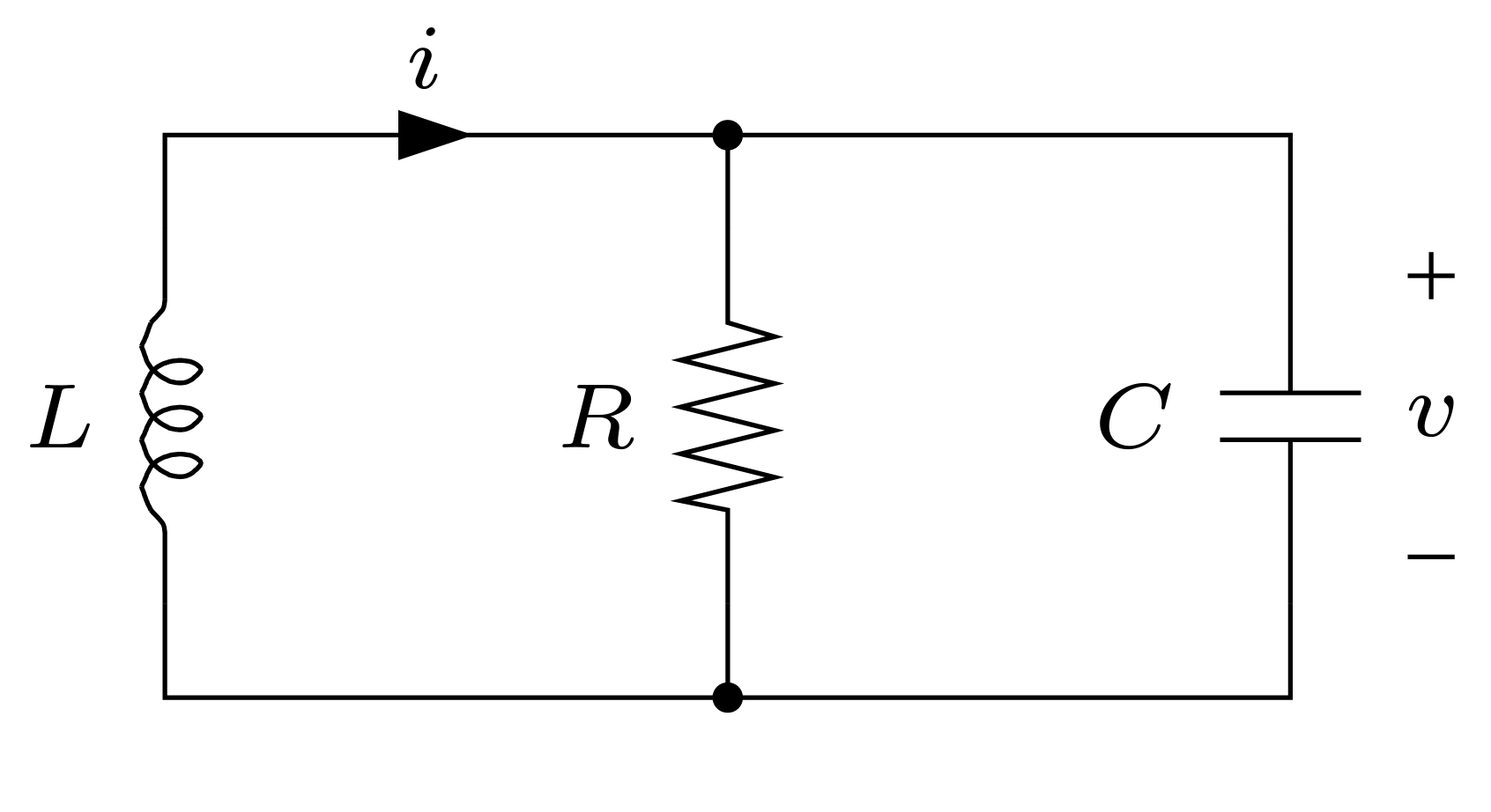
Parallel RCL circuit - resistor R in parallel with inductor L and capacitor C. The supplied voltage is the voltage across the capacitor v and the current is the current flowing the the inductor. — Fig. 76 Parallel RLC circuit (reproduced from page 6-8 of [Boyd, 1993])#

Solution to example 2#

We have

(51)#

v (t) = - L \frac{d i (t)}{d t}

and

(52)#

C \frac{d v (t)}{d t} = i (t) - \frac{v (t)}{R}

Integrating both sides of (51) we get

(53)#

\int_{0}^{t} v (τ) d τ = - L i (t)

We rewrite (53) as

(54)#

i (t) = - \frac{1}{L} \int_{0}^{t} v (τ) d τ

Substituting (54) into (52) we eliminate $i (t)$ and obtain

(55)#

C \frac{d v (t)}{d t} = - \frac{1}{L} \int_{0}^{t} v (τ) d τ - \frac{v (t)}{R}

Taking the derivative of both sides of (55) and gathering terms yields the differential equation

(56)#

\frac{d^{2} v (t)}{d t^{2}} + \frac{1}{R C} \frac{d v (t)}{d t} + \frac{1}{L C} v (t) = 0

Laplace transforms#

Taking Laplace transforms of ((56)) we have

(57)#

(s^{2} V (s) - s v (0) - v^{'} (0)) + \frac{1}{R C} (s V (s) - v (0)) + \frac{1}{L C} V (s) = 0

Assuming $v^{'} (0) = 0$ , then (57) becomes

(58)#

(s^{2} + \frac{1}{R C} s + \frac{1}{L C}) V (s) = (s + \frac{1}{R C}) v (0)

Let $v (0) = k$ (a constant), we can represent (58) as the rational function

(59)#

V (s) = \frac{k (s + \frac{1}{R C})}{s^{2} + \frac{1}{R C} s + \frac{1}{L C}}

And we can now take the partial fraction expansion of $V (s)$ and take the inverse Laplace transform to arrive at a solution for $v (t)$ .

Types of response#

The roots of the denominator of (59) are given by

\begin{array}{r} \begin{aligned} λ & = \frac{- \frac{1}{R C} \pm \sqrt{{(\frac{1}{R C})}^{2} - \frac{4}{L C}}}{2} \\ = - \frac{1}{2 R C} \pm \sqrt{\frac{1}{4 R^{2} C^{2}} - \frac{1}{L C}} \end{aligned} \end{array}

There are four possible types of response that would result from this quadratic.

Which type occurs depends on the discriminant of the quadratic formula:

\frac{1}{4 R^{2} C^{2}} - \frac{1}{L C}

The discriminant depends on the relative values of $L$ , $C$ and $R$ .

The four types are discussed below

Type 1: Overdamped response
Type 2: Critically damped response
Type 3: Underdamped response
Type 4: Undamped response

Type 1: Overdamped response#

If the discriminant is positive

\frac{1}{L C} < \frac{1}{4 R^{2} C^{2}}

and the roots $λ_{1}$ and $λ_{2}$ will be real and distinct. The voltage $v (t)$ will be the sum of two exponential decays

v (t) = r_{1} e^{- λ_{1} t} + r_{2} e^{- λ_{2} t}

where $r_{1}$ and $r_{2}$ are the residues of the partial-fraction expansion of (59).

Type 2: Critically damped response#

If the discriminant is zero

\frac{1}{L C} = \frac{1}{4 R^{2} C^{2}}

the roots $λ_{1}$ and $λ_{2}$ will be real and equal to $λ = - 1 / (2 R C)$ . The voltage $v (t)$ will be

v (t) = r_{1} t e^{- λ t} + r_{2} e^{- λ t}

Again, $r_{1}$ and $r_{2}$ are the residues of the partial-fraction expansion of (59).

Type 3: Underdamped response#

If the discriminant is negative then

\frac{1}{L C} > \frac{1}{4 R^{2} C^{2}}

and

λ_{1, 2} = - \frac{1}{2 R C} \pm j \sqrt{\frac{1}{L C} - \frac{1}{4 R^{2} C^{2}}}

giving

σ = - \frac{1}{2 R C}

and

ω = \sqrt{\frac{1}{L C} - \frac{1}{4 R^{2} C^{2}}}

This will be a decaying sinusoidal waveform and means that

Q = \frac{R}{\sqrt{L / C}}

and

ζ = \frac{\sqrt{L / C}}{2 R}

Type 4: Undamped response#

If the resistance $R$ is infinite, the real part $σ =$ and the poles $λ_{1}$ and $λ_{2}$ are imaginary. The energy in the circuit will continually flow backwards and forwards between the inductor and the capacitor. This will result in a sinusoidal response $v (t) = α \cos (ω t + ϕ)$ . The actual values of amplitude $α$ and phase $ϕ$ again depend on the residues of the partial expansion of (59).

Interpretation of $Q$ #

$Q$ is a neasure of the number of cycles to decay

Time to decay to 1% of amplitude us about $4.6 / | σ |$
The period of oscilation is $2 π / ω$
The number of cycles to decay to 1% amplitude

N_{1 %} \approx \frac{4.6 / | σ |}{2 π / ω} = 1.46 \frac{ω}{2 | σ |}

A rule of thumb (accurate for $Q > 2$ or so):

N_{1 %} \approx 1.46 Q

Another rule of thumb: $N_{4 %} \approx Q$

Example 3#

Assume $ω = 2 π$ rad/s (so period $T = 1$ s). Plot the response $e^{- σ t} \cos (ω t)$ for $Q = 20$ and $Q = 10$ .

Solution to example 3#

Given that

Q = \frac{1}{2} \sqrt{\frac{ω^{2} + σ^{2}}{σ^{2}}}

it is relatively easy to show that

σ = \frac{ω}{\sqrt{4 Q^{2} - 1}}

So to plot this:

omega = 2*pi;
t = linspace(0,30,1000);
Q = 20;
sigma = omega/sqrt(4*Q^2 - 1);
subplot(211)
plot(t,exp(-sigma*t).*cos(omega*t)),title('Q = 20'),grid on
Q = 10;
sigma = omega/sqrt(4*Q^2 - 1);
subplot(212)
plot(t,exp(-sigma*t).*cos(omega*t)),title('Q = 10'), grid on

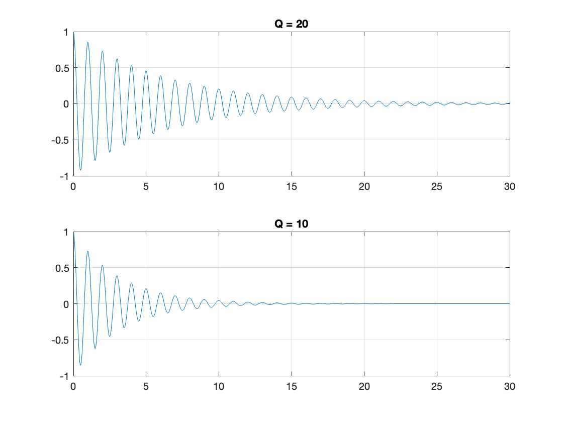
../_images/f4d9889a3dd3c62da9190b73e0a2e6f8a363beacaf4fbbdb471f90b4a336a01f.png

../_images/0035cded96b37b286f94b0ec07544b825d8a703e6a47c881bf95440b5b5503a2.png

The MATLAB code to reproduce this figure is given in example3.mlx

Dominant Poles#

Suppose the poles of $F (s)$ are $p_{1}, \dots, p_{n}$ . The asymptotic growth (or decay if $< 0$ ) is determined by the maximum real part:

α = max {ℜ p_{1}, \dots, ℜ p_{n}}

The pole (pr poles) which achieve this maximum real part are called dominant

As $t \to \infty$ these terms become larger and larger compared to the other terms, no matter what the residues.

As an example, see Fig. 77. Although this system has six poles, the pole closest to $s = 0$ has the largest real part and so will be dominant.

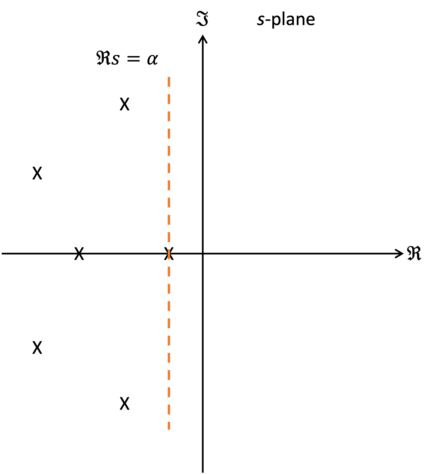
Illustration of a dominant pole — Fig. 77 Dominant poles in a transform $F (s)$ #

Example 4#

Let

F (s) = \frac{100}{s + 2} + \frac{1}{s + 1}

From transform tables

f (t) = 100 e^{- 2 t} + e^{- t}

The assympotic decay rate is determined by the pole at $s = - 1$
Assymptotically, $f (t)$ decays like $e^{- t}$
Even though the residue associated with for the nondominant pole is 100 times larger, the term associated with the dominant pole is larger for $t > 4.6$ .

t = linspace(0,10,1000);
f1 = 100*exp(-2*t);
f2 = exp(-t);
subplot(2,2,1)
plot(t,f1),grid,ylim([0,0.5]),xlim([0,10])
subplot(2,2,2)
plot(t,f2),ylim([0,0.5]),grid
subplot(2,2,[3,4])
plot(t,f1+f2),ylim([0,0.5]),grid

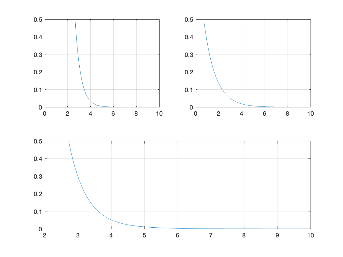
../_images/56ae2dcc3b7e87e800e40aa941d8f2dfd91c27cd0616d6c69ef2b713b00b4990.png

The MATLAB code to reproduce this figure is given in example4.mlx

Stability of autonomous LCCODEs#

The linear constant coefficient ordinary differential equation (LCCODE)

a_{n} \frac{d^{n} y (t)}{d t^{n}} + a_{n - 1} \frac{d^{n - 1} y (t)}{d t^{n - 1}} + \dots + a_{0} y (t) = 0

is stable if all solutions converge to zero, regardless of initial condition.

Take the Laplace transform

\begin{array}{r} \begin{matrix} a_{n} (s^{n} Y (s) - s^{n - 1} y (0) - s^{n - 2} y^{'} (0) - \dots - y^{(n - 1)} (0)) \\ + a_{n - 1} (s^{n - 1} Y (s) - s^{n - 2} y (0) - \dots - y^{(n - 2)} y (0)) \\ + \dots + a_{0} y (0) = 0 \end{matrix} \end{array}

Y (s) = \frac{b_{n - 1} s^{n - 1} + b_{n - 2} s^{n - 2} + \dots + b_{1} s + b_{0}}{a_{n} s^{n} + a_{n - 1} s^{n - 1} + \dots + a_{1} s + a_{0}} = \frac{b (s)}{a (s)}

where $b (s)$ depends on the initial conditions.

The LCCODE is stable only when all poles of $Y (s)$ have negative real part, i.e. the roots of $a (s)$ are in the left half plane.

Initial value theorem#

A general property of Laplace transforms (not just for rational $F (s)$ :

lim_{s \to \infty} s F (s) = f (0^{+})

(We can take $s$ to be real in the limit).

This makes a connection between $f (t)$ for small $t$ and $F (s)$ for large $s$ .

Reason: for large (real) $s$ , $s e^{- s t}$ is bunched up near $t = 0$ , so:

F (s) = \int_{0}^{\infty} s e^{- s t} f (t) d t \approx f (0^{+}) \int_{0}^{\infty} s e^{- s t} d t = f (0^{+})

Examples 5#

a) Find the initial value of $f (t) = e^{a t}$

b) Find the initial value of the unit step signal $u_{0} (t)$

Solutions to examples 5#

a) For $f (t) = e^{a t}$ , $F (s) = 1 / (s - a)$ so

lim_{s \to \infty} s F (s) = lim_{s \to \infty} \frac{s}{s - a} = 1 = f (0^{+})

b) For $f (t) = u_{0} (t)$ , $F (s) = 1 / s$

lim_{s \to \infty} s F (s) = 1 = f (0^{+})

Final value theorem#

The final value theorem make the connection between $f (t)$ for large $t$ and $F (s)$ for small $s$ .

lim_{t \to \infty} f (t) = {s F (s) |}_{s = 0}

if the limit exists.

Reason: from the relation between Laplace transforms and derivatives,

s F (s) - f (0) = L {\frac{d f (t)}{d t}} = \int_{0}^{\infty} \frac{d f (t)}{d t} e^{- s t} d t

s {F (s) |}_{s = 0} - f (0) = \int_{0}^{\infty} \frac{d f (t)}{d t} d t = lim_{t \to \infty} f (t) - f (0)

s {F (s) |}_{s = 0} = lim_{t \to \infty} f (t)

Examples 6#

a) Find the final value of $f (t) = 1 - e^{- t}$

b) Find the final value of $f (t) = \cos (ω t)$

Solutions to examples 6#

a) If $f (t) = 1 - e^{- t}$ ,

F (s) = \frac{1}{s} - \frac{1}{s + 1},

and

lim_{t \to \infty} f (t) = {s F (s) |}_{s = 0} = \frac{s}{s} - \frac{s}{s + 1} = 1 - \frac{0}{1} = 1

b) $f (t) = \cos (ω t)$ and

F (s) = \frac{s}{s^{2} + ω^{2}}

In this case $lim_{t \to \infty} f (t)$ does not exist; the final value theorem does not apply here.

Summary#

In this unit we have presented some properties of rational polynomials which apply to the Laplace transform of signals and systems represented by transfer functions. In particular, we have developed some tools that help us to reason about the behaviour of a signal or system providing we know the location of its poles and zeros.

We covered the following topics

Inverse Laplace transform of a rational F(s)
Qualitative properties of terms
Quantitative properties of terms
Complex poles: Damping ratio \zeta and quality factor Q
Dominant Poles
Stability of autonomous LCCODEs
Initial value theorem
Final value theorem

Unit 5.1: Take Aways#

Inverse Laplace transform terms#

The poles of $F (s)$ determine the types of terms that appear in $f (t)$
The zeros (or residues) of $F (s)$ determine the coeficients multiplying each term, or the amplitude and phase of oscillitory terms.

Qalitative properties of terms#

Section Qualitative properties of terms summarizes the types of responses that $f (t)$ (a signal or system whose Laplace transform is a rational polynomial $F (s)$ [3]) can exhibit.
The growth-rate and decay-rate of each system response term is governed by the real part of the pole $σ$ .
- A response term will grow if $σ > 0$
- A response term will decay if $σ < 0$
If the poles are complex, the frequency of the sinusoidal response term will be the imaginary part of the pole $ω$ rad/s
The response term will be a pure sinusoid if $σ = 0$ and the poles are imaginary.

Quantative properties of terms#

For complex poles, there are two measures of the decay rate per cycle of oscillation. These are defined in Complex poles: Damping ratio \zeta and quality factor Q.

In Example 2: parallel RLC circuit we introduced the concepts of overdamped response, critically damped response*, underdamped response and undamped response. We also provided the definitions for $Q$ and $ζ$ for this circuit.

Interpretation of Q#

In Interpretation of Q we declared that the time to decay to 1% of amplitude (called settling time) is about $4.6 / | σ |$ and the number of cycles to decay to 1% amplitude is about $N_{1 %} = 1.46 ω / (2 | σ |)$ s. $N_{1 %} \approx 1.46 Q$ s for $Q > 2$ .

We also stated that $N_{4 %} \approx Q$ s.

Dominant poles#

The dominant poles of a system are those which have the largest real part $σ$ . The response term associated with this pole (or pole pair) will eventually come to dominate the overall response $f (t)$ .

Stability of LTI systems#

An LTI system can be represented as an LCCODE.

Such systems will be stable if all the poles have negative real part. Such poles will lie in the left-hand-plane of the $s$ -plane.
By the counter argument, a system which has any poles that have positive real part will be unstable.
If a complex pole and its conjugate is on the imaginary axis the response will be sinusoidal. We call systems with this property marginally stable.
If a pole is real and zero, it will lie at the origin $s = 0$ of the $s$ -plane. The corresponding term’s response will be a constant value $f (t) = a$ .
If there are two poles are the origin of the $s$ -plane, the corresponding term’s response would be $f (t) = a t$ .

Consequences of what we have learned#

Knowledge of the dominant poles, the quantative properties, damping ratio $ζ$ and quality factor $Q$ enable us to evaluate the stability and likely response of a system without needing to compute the actual response.

Initial value and final value theorem#

The initial value and final value properties of the Laplace transform allow us to compute the initial value and final value of $f (t)$ using knowledge of the transform $F (s)$ .

Still to come#

In the next unit Unit 5.2: More on the Qualitative and Quantitative Response of First- and Second-Order Poles we will expand our knowledge of the response of a complex term by defining a canonical model of a quadratic pole. We will also do some examples to practice what we have learned in this unit.

We will build on these ideas in EG-247 Digital Signal Processing and you will be able to use what you have learned in EG-243 Control Systems.

References#

[All24]

Chad Allie. Transfer function analysis of dynamic systems. 2024. Retrieved April 3, 2024. URL: MathWorks-Teaching-Resources/Transfer-Function-Analysis-of-Dynamic-Systems.

[Boy93] (1,2)

Stephen Boyd. Ee-102: introduction to signals and systems. 1993. Retrieved April 3, 2024. URL: https://web.stanford.edu/~boyd/ee102/.

Unit 5.1: Qualitative Properties of Signals and Transfer functions

Contents

Unit 5.1: Qualitative Properties of Signals and Transfer functions#

Acknowledgements#

Agenda#

Inverse Laplace transform of a rational F(s)#

Qualitative properties of terms#

Real poles#

Complex poles#

Imaginary poles#

Repeated poles#

Quantitative properties of terms#

Example 1#

Qualitative analysis from the pole-zero map#

Complex poles: Damping ratio ζ and quality factor Q#

Example 2: parallel RLC circuit#

Solution to example 2#

Laplace transforms#

Types of response#

Type 1: Overdamped response#

Type 2: Critically damped response#

Type 3: Underdamped response#

Type 4: Undamped response#

Interpretation of Q#

Example 3#

Solution to example 3#

Dominant Poles#

Example 4#

Stability of autonomous LCCODEs#

Initial value theorem#

Examples 5#

Solutions to examples 5#

Final value theorem#

Examples 6#

Solutions to examples 6#

Summary#

Unit 5.1: Take Aways#

Inverse Laplace transform terms#

Qalitative properties of terms#

Quantative properties of terms#

Interpretation of Q#

Dominant poles#

Stability of LTI systems#

Consequences of what we have learned#

Initial value and final value theorem#

Still to come#

References#

Footnotes#

Inverse Laplace transform of a rational $F (s)$ #

Complex poles: Damping ratio $ζ$ and quality factor $Q$ #

Interpretation of $Q$ #