Unit 3.1: Response of a Continuous-Time LTI System and the Convolution Integral

This section is based on Section 2.1 of [Hsu, 2020].

Follow along at cpjobling.github.io/eg-150-textbook/lti_systems/lti1

Subjects to be Covered

• A. Impulse Response

• B. Response to an Arbitrary Input

• C. Convolution Integral

• D. Properties of the Convolution Integral

• E. Convolution Integral Operation

• F. Step Response

• Exercises 5: Responses of a Continuous-Time LTI System and Convolution

A. Impulse Response

The impulse response \(h(t)\) of a continuous-time LTI system (represented by \(\mathbf{T}\)) is defined as the response of the system when the input is \(\delta(t)\), that is,

\[h(t) = \mathbf{T}\left\{\delta(t)\right\}\]

B. Response to an Arbitrary Input

From the Sifting Property

\[\int_{-\infty}^{\infty}f(t)\delta(t-\alpha)dt=f(\alpha)\]

an arbitrary continuous-time input can be expressed in terms of the Dirac delta function as

\[x(\tau) = \int_{-\infty}^{\infty}x(\tau)\delta(t-\tau)d\tau = x(t)\]

Since the system is linear, the response \(y(t)\) of the system with arbitrary input \(x(t)\) can be expressed as

\[y(t) = \mathbf{T}\left\{x(t)\right\} = \mathbf{T}\left\{\int_{-\infty}^{\infty}x(\tau)\delta(t-\tau)\,d\tau\right\}\]

\[ = \int_{-\infty}^{\infty}x(t)\mathbf{T}\left\{\delta(t - \tau)\right\}\]

Since the system is time-invariant, we have

\[h(t-\tau)=\mathbf{T}\left\{\delta(t-\tau)\right\}\]

Substituting \(h(t-\tau)\) into the equation for \(y(t)\) gives

\[y(t) = \int_{-\infty}^{\infty}x(\tau)h(t-\tau)\,d\tau\]

This equation indicates that a continuous-time LTI system is completely characterised by its impulse response \(h(t)\).

C. Convolution Integral

The equation

\[y(t) = \int_{-\infty}^{\infty}x(\tau)h(t-\tau)\,d\tau\]

defines the convolution of two continuous-time signals \(x(\tau)\) and \(h(t)\) denoted by

\[y(t) = x(t) * h(t) = \int_{-\infty}^{\infty}x(\tau)h(t-\tau)\,d\tau\]

The equation

\[y(t) = x(t) * h(t) = \int_{-\infty}^{\infty}x(\tau)h(t-\tau)\,d\tau\]

is commonly called the convolution integral.

Thus we have the fundamental result that:

the output of any continuous-time LTI system is the convolution of the input \(x(t)\) with the impulse response \(h(t)\) of the system.

Fig. 34 illustrates the definition of the impulse response \(h(t)\) and the convolution integral.

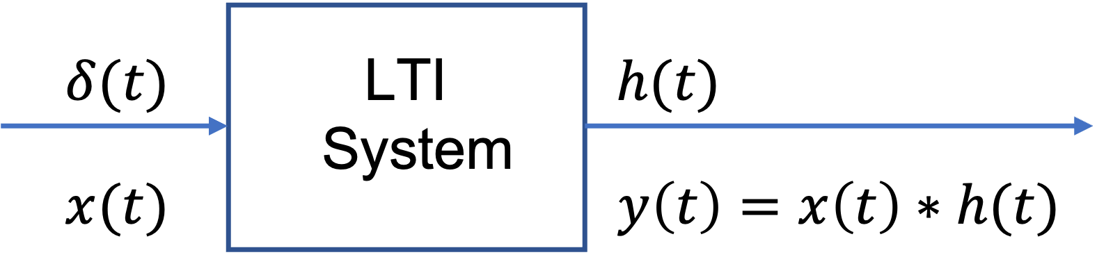
Fig. 34 Continuous-time LTI system

D. Properties of the Convolution Integral

The convolution integral has the following properties.

1. Commutative:

\[x(t) * h(t) = h(t) * x(t)\]

2. Associative:

\[\left\{x(t) * h_1(t)\right\} * h_2(t) = x(t) * \left\{h_1(t) * h_2(t)\right\}\]

3. Distributive:

\[x(t)*\left\{h_1(t) + h_2(t)\right\} = x(t)*h_1(t) + x(t)*h_2(t)\]

E. Convolution Integral Operation

Applying the communitative propery of convolution to the convolution integral, we obtain

\[y(t) = h(t) * x(t) = \int_{-\infty}^{\infty}h(\tau)x(t-\tau)\,d\tau\]

which may at times be easier to evaluate than

\[y(t) = x(t) * h(t) = \int_{-\infty}^{\infty}x(\tau)h(t-\tau)\,d\tau\]

Graphical Evaluation of the Convolution Integral

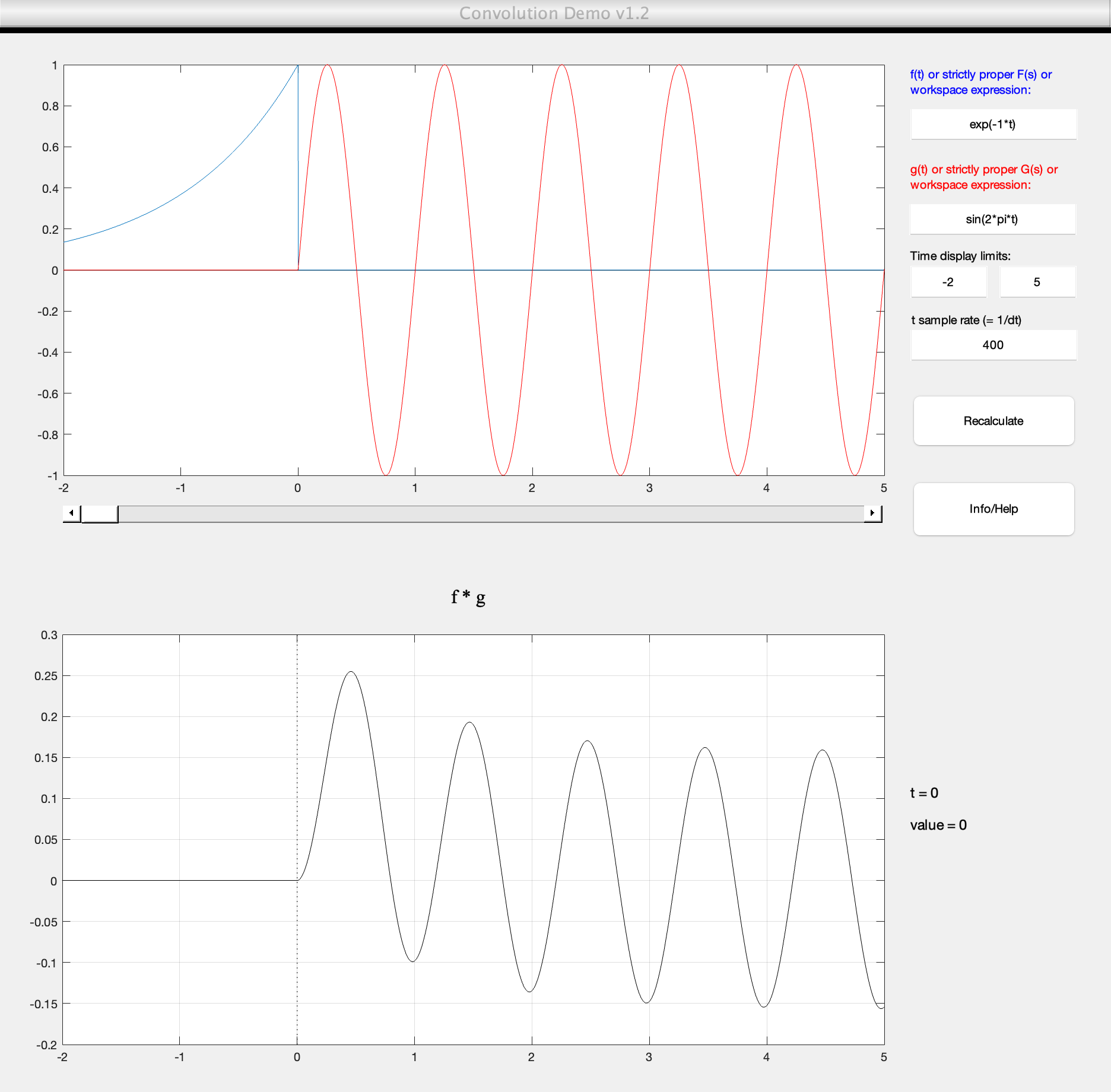
The convolution integral is most conveniently evaluated by a graphical evaluation. We give three examples (5.4—5.6) which we will demonstrate in class using a graphical visualization tool developed by Teja Muppirala of the Mathworks and updated by Rory Adams.

The tool: convolutiondemo.m (see license.txt).

We will then work through the examples again in the examples class.

cd matlab/convolution_demo
dir
convolutiondemo

.                  README.md          license.txt        
..                 convolutiondemo.m  

Warning: The EraseMode property is no longer supported and will error in a future release.

> In convolutiondemo>convolutiondemo_LayoutFcn (line 398)
In convolutiondemo>gui_mainfcn (line 1181)
In convolutiondemo (line 44)

convolutiondemo % ignore warnings

Summary of Steps

1. The inpulse response \(h(\tau)\) is time reversed (that is, reflected about the origin) to obtain \(h(-\tau)\) and then shifted by \(t\) to form \(h(t-\tau) = h\left[-(\tau - t)\right]\), which is a function of \(\tau\) with parameter \(t\).

2. The signal \(x(\tau)\) and \(h(t-\tau)\) are multiplied together for all values of \(\tau\) with \(t\) fixed at some value.

3. The product \(x(\tau)h(t-\tau)\) is integrated over all \(\tau\) to produce a single output value \(y(t)\).

4. Steps 1 to 3 are repeated as \(t\) varies over \(-\infty\) to \(\infty\) to produce the entire output \(y(t)\).

Examples of the above convolution integral operation are given in Examples 5.4 to 5.6.

Example

We will do Exercise 5.4 in class

F. Step Response

The step response \(s(t)\) of a continuous-time LTI system (represented by \(\mathbf{T}\)) is defined by the response of the system when the input is \(u_0(t)\); that is,

\[s(t) = \mathbf{T}\left\{u_0(t)\right\}\]

In many applications, the step response \(s(t)\) is also a useful characterisation of the system. The step response can be easily determined using the convolution integral; that is,

\[s(t) = h(t)*u_0(t) = \int_{-\infty}^{\infty} h(\tau)u_0(t-\tau)\,d\tau = \int_{0}^{t} h(\tau)\,d\tau\]

Thus the step response \(s(t)\) can be obtained by integrating the impulse response \(h(t)\).

Impulse response from step response

Differentiating the step response with respect to \(t\), we get

\[h(t) = s'(t) = \frac{ds(t)}{dt}\]

Thus the impulse response \(h(t)\) can be determined by differentiating the step response \(s(t)\).

Exercises 5: Responses of a Continuous-Time LTI System and Convolution

Exercise 5.1

Verify the following properties of the convolution integral; that is,

(a) \(x(t)*h(t) = h(t)*x(t)\)

(b) \(\left\{x(t) * h_1(t)\right\} * h_2(t) = x(t)*\left\{h_1(t) * h_2(t)\right\}\)

For the answer, refer to the lecture recording or see solved problem 2.1 in in [Hsu, 2020].

Exercise 5.2

Show that

(a) \(x(t) * \delta(t) = x(t)\)

(b) \(x(t) * \delta(t-t_0) = x(t - t_0)\)

(c) \(x(t)*u_0(t) = \int_{-\infty}^{t}x(\tau)\,d\tau\)

(d) \(x(t) * u_0(t - t_0) = \int_{-\infty}^{t_0}x(\tau)\,d\tau\)

For the answer, refer to the lecture recording or see solved problem 2.2 in in [Hsu, 2020].

Exercise 5.3

Let \(y(t) = x(t) * h(t)\). Then show that

\[x(t-t_1)*h(t-t_2) = y(t - t_1 - t_2)\]

For the answer, refer to the lecture recording or see solved problem 2.3 in in [Hsu, 2020].

Exercise 5.4

The input \(x(t)\) and the impulse response \(h(t)\) of a continuous-time LTI system are given by

\[x(t) = u_0(t)\]

\[h(t) = e^{-\alpha t}u_0(t),\;\alpha > 0\]

(a) Compute the output \(y(t)\) by using the convolution integral

\[y(t) = x(t) * h(t) = \int_{-\infty}^{\infty}x(\tau)h(t-\tau)\,d\tau\]

(b) Compute the output \(y(t)\) by using the convolution integral

\[y(t) = h(t) * x(t) = \int_{-\infty}^{\infty}h(\tau)x(t-\tau)\,d\tau\]

Solutions

(a) Graphical

Using the convolutiondemo tool chose a value for \(\alpha\). I will use \(\alpha = 1\).

Then set f(t), which represents \(x(t)\), to heaviside(t) and g(t). which represents \(h(t)\) to exp(-1*t)

Manual solution

For the manual solution, refer to the lecture recording or see solved problem 2.3 in in [Hsu, 2020].

MATLAB Solution

We can also use the Symbolic Math Toolbox to solve the problem directly:

syms t tau alpha
assume(alpha > 0)

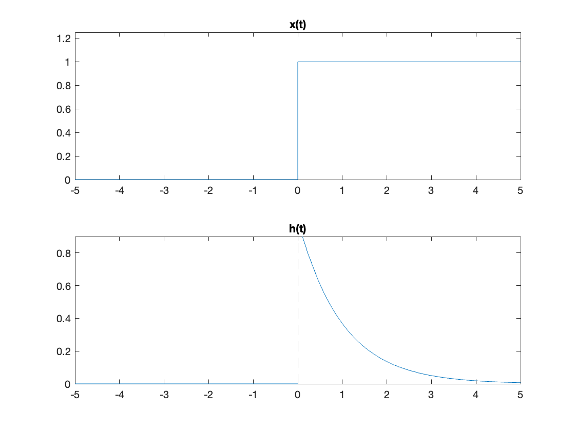
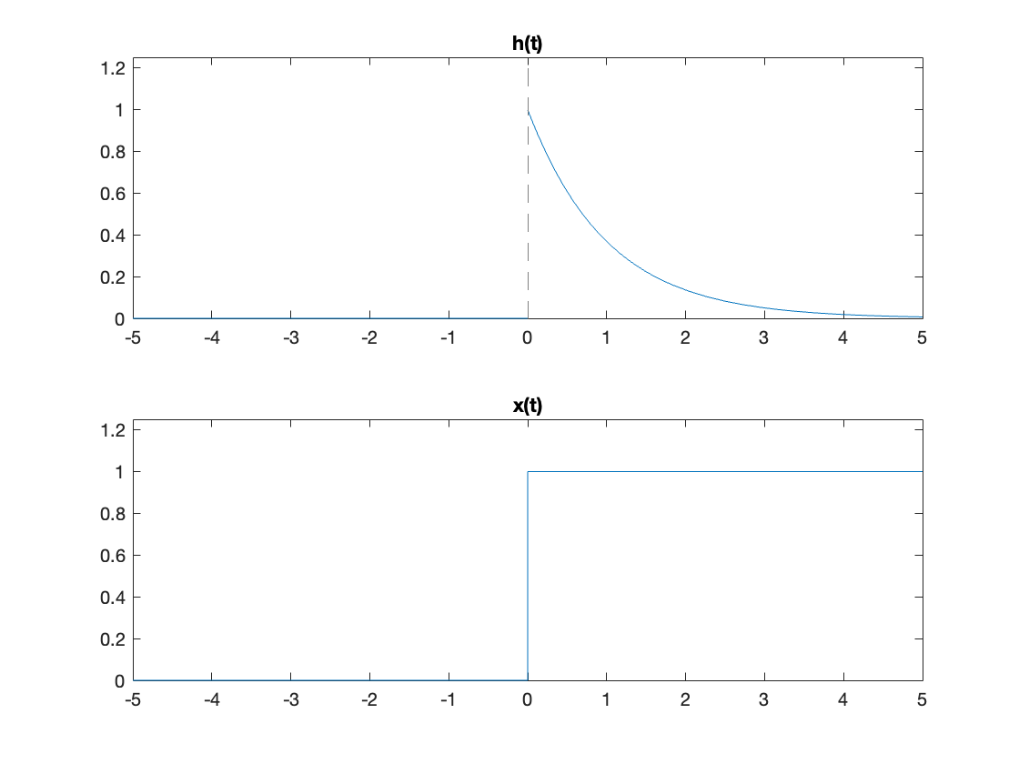
x(t) = heaviside(t); % unit step function
subplot(211)
fplot(x(t)),title('x(t)'),ylim([0,1.25])
h(t) = exp(-alpha*t)*heaviside(t);
subplot(212)
fplot(subs(h(t),alpha,1)),title('h(t)')

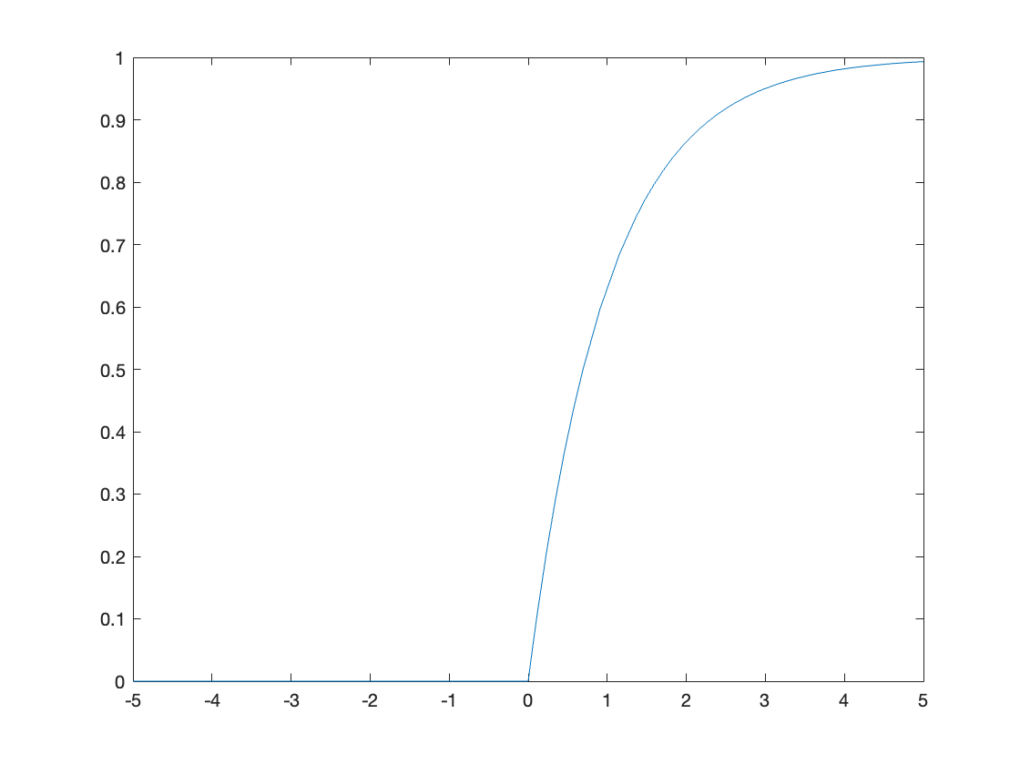
Compute \(y(t)\) using the MATLAB function int to compute the convolution integral symbolically.

y(t) = int(x(tau)*h(t - tau),tau,0,t)

y(t) =

-(2*exp(-(alpha*t)/2)*(exp(-(alpha*t)/2)/2 - exp((alpha*t)/2)/2)*(sign(t)/2 + 1/2))/alpha

Plot the result for \(\alpha = 1\)

ya(t) = subs(y(t),alpha,1)
fplot(ya(t))

ya(t) =
 

-2*exp(-t/2)*(exp(-t/2)/2 - exp(t/2)/2)*(sign(t)/2 + 1/2)

(b) Graphical

Reverse the settings for f(t)and g(t) in the convolutiondemo tool.

Manual solution

For the manual solution, refer to the lecture recording or see solved problem 2.3 in in [Hsu, 2020].

MATLAB Solution

Reverse the arguments to the fplot and int functions.

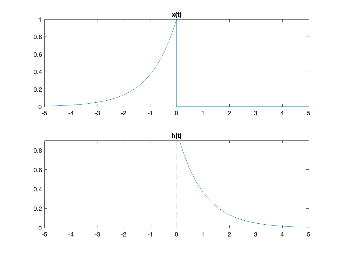
subplot(211)
fplot(subs(h(t),alpha,1)),title('h(t)'),ylim([0,1.25])
subplot(212)
fplot(x(t)),title('x(t)'),ylim([0,1.25])

y(t) = int(h(tau)*x(t - tau),tau,-Inf,Inf)

y(t) =
 

-(2*exp(-(alpha*t)/2)*(exp(-(alpha*t)/2)/2 - exp((alpha*t)/2)/2)*(sign(t)/2 + 1/2))/alpha

Plot the result for \(\alpha = 1\)

yb(t) = subs(y(t),alpha,1)
fplot(yb(t))

yb(t) =

-2*exp(-t/2)*(exp(-t/2)/2 - exp(t/2)/2)*(sign(t)/2 + 1/2)

Go back to F. Step Response

Exercise 5.5

Compute the output \(y(t)\) for a continuous-time LTI system whose impulse response \(h(t)\) and the input \(x(t)\) are given by

\[h(t) = e^{-\alpha t}u_0(t)\]

\[x(t) = e^{\alpha t}u_0(-t)\]

\[\alpha > 0.\]

Solutions

Manual solution

For the manual solution, refer to the lecture recording or see solved problem 2.3 in in [Hsu, 2020].

MATLAB Solution

We can also use the Symbolic Math Toolbox to solve the problem directly:

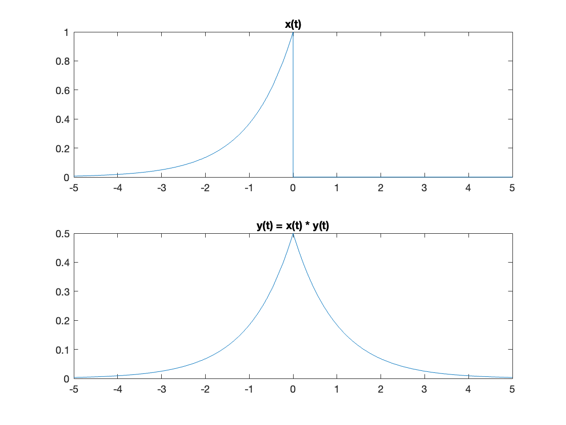
x(t) = exp(t)*heaviside(-t);
subplot(211)
fplot(x(t)),,title('x(t)')
h(t) = exp(-1*t)*heaviside(t);
subplot(212)
fplot(h(t)),title('h(t)')

Compute \(y(t)\) using the convolution integral

y(t) = int(x(tau)*h(t - tau),tau,-Inf,Inf)

y(t) =
 

piecewise(0 <= t, exp(-t)/2, t <= 0, exp(t)/2)

Plot the result for \(\alpha = 1\)

fplot(y(t)),title('y(t) = x(t) * y(t)')

Exercise 5.6

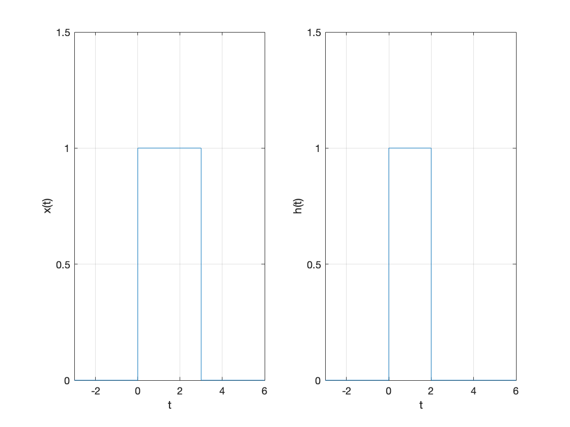
Evaluate \(y(t) = x(t) * h(t)\), where \(x(t)\) and \(h(t)\) are shown in Fig. 35, by an alalytical technique, and (b) by a graphical method.

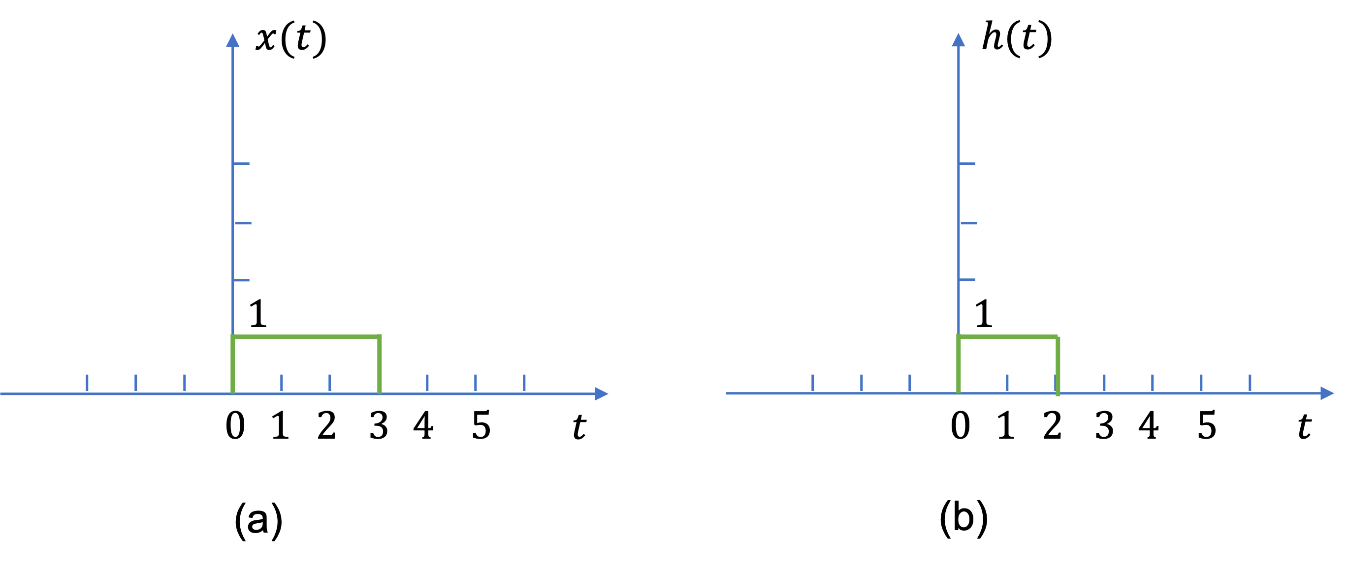
Fig. 35 Signal and system for example 5.6

Solutions

(a) Analytical

We first express \(x(t)\) and \(h(t)\) in functional form using the unit step (or Heaviside function)

\[x(t) = u_0(t) - u_0(t-3)\]

\[h(t) = u_0(t) - u_0(t-2)\]

We will use the MATLAB Symbolic Math Toolbox:

x(t) = heaviside(t)-heaviside(t-3);
h(t) = heaviside(t)-heaviside(t-2);
subplot(121)
fplot(x(t),[-3,6]),grid,ylim([0,3]),ylabel('x(t)'),xlabel('t')
subplot(122)
fplot(h(t),[-3,6]),grid,ylim([0,3]),ylabel('h(t)'),xlabel('t')

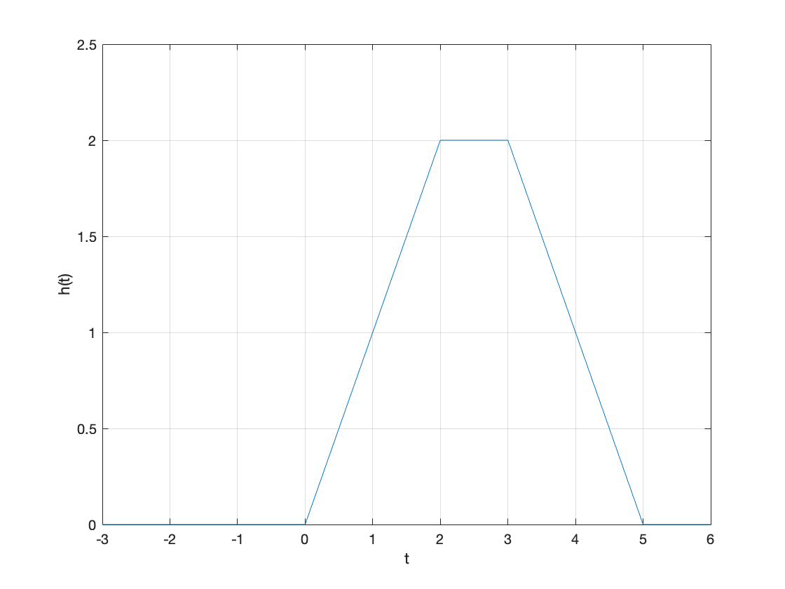
Compute \(y(t)\)

y(t) = int(x(tau)*h(t - tau),tau,-Inf,Inf)

y(t) =
 

heaviside(t - 5)*(t - 5) - heaviside(t - 3)*(t - 3) - heaviside(t - 2)*(t - 2) + t*heaviside(t)

Plot the result

fplot(y(t),[-3,6]),grid,ylim([0,2.5]),ylabel('h(t)'),xlabel('t')

(b) Graphical

Since both functions are unity between the limits set by the Heaviside function, graphical solution requires multiple applications of the definate integral

\[\int_{t_0}^{t_1}1\times 1\,d\tau = \int_{t_0}^{t_1}1\,d\tau\]

with different values for the limits \(t_0\) and \(t_1\). The convolutiondemo tool can help us discover the limits for the piecewise continuous signal \(y(t)\).

For the complete solution to Example 5.2 refer to the lecture recording or see solved problem 2.6 in in [Hsu, 2020].

Summary

In this lecture we have looked at

• B. Response to an Arbitrary Input

• C. Convolution Integral

• D. Properties of the Convolution Integral

• E. Convolution Integral Operation

• F. Step Response

Unit 3.1: Take Aways

• Impulse response: \(h(t) = \mathbf{T}\left\{\delta(t)\right\}\)

• Step response: \(s(t) = \mathbf{T}\left\{u_0(t)\right\} = \int_0^t h(\tau)\,d\tau\)

• Arbitrary system response: \(y(t) = \int_{-\infty}^{\infty} x(t)h(t-\tau)\,d\tau\)

• Convolution itegral: \(y(t) = x(t)*h(t) = \int_{-\infty}^{\infty} x(t)h(t-\tau)\,d\tau = \int_{-\infty}^{\infty} x(t-\tau)h(\tau)\,d\tau\)

• Properties of the convolution integral:

  • Communitative: \(x(t) * h(t) = h(t) * x(t)\)

  • Associative: \(\left\{x(t) * h_1(t) \right\} * h_2(t) = x(t)*\left\{h_1(t) * h_2(t) \right\}\)

  • Distributive: \(x(t)*\left\{h_1(t) + h_2(t)\right\} = x(t)*h_1(t) + x(t) * h_2(t)\)

• The convolution integral can be computed graphically or analytically.

Next Time

We continue our introduction to continuous-time LTI system by considering

• Properties of Continuous-Time LTI Systems

• Eigenfunctions of Continuous-Time LTI Systems

References

Hsu20(1,2,3,4,5,6,7,8)

Hwei P. Hsu. Schaums outlines signals and systems. McGraw-Hill, New York, NY, 2020. ISBN 9780071634724. Available as an eBook. URL: https://www.accessengineeringlibrary.com/content/book/9781260454246.