Unit 3.2: Properties and Eigenfunctions of Continuous-Time LTI Systems#
This section is based on Sections 2.3 and 2.4 of [Hsu, 2020]
Follow along at cpjobling.github.io/eg-150-textbook/lti_systems/lti2

Subjects to be covered#
We continue our introduction to continuous-time LTI systems by considering:
Properties of Continuous-Time LTI Systems#
A. Systems with or without memory#
Since the output \(y(t)\) of a memoryless system depends only on the current input \(x(t)\), then, if the system is also linear and time-invariant, this relationship can only be of the form
where \(K\) is a (gain) constant.
Thus the corresponding impulse response \(h(t)\) is simply
Therefore, if \(h(t_0) \neq 0\) for \(t_0 \neq 0\), then the continuous-time LTI system has memory.
B. Causality#
Causal continuous-time LTI systems#
As discussed in Section Causal and Non-Causal Systems, a causal system does not respond to an input event until that event actually occurs.
Therefore, for a causal LTI system, we have
Applying the causality condition to the convolution integral, the output of a causal continuous-time LTI system is expressed as
Alternatively, applying the causality to the convolution integral (defined in Section C. Convolution Integral)
we have
This equation shows that the only values of the input \(x(t)\) used to evaluate the output \(y(t)\) are those for \(\tau \le t\).
Causal signals#
Based on the causality condition, any signal is called causal if
and is called anticausal if
Combining the definition of a causal signal with a causal system, when the input \(x(t)\) is causal, the output of a causal continuous-time LTI system is given by
C. Stability#
The BIBO (bounded-input/bounded-output) stability of an LTI system (Section Stable Systems) is readily ascertained by the impuse response. It can be shown (Exercise 6.5) that a continuous-time LTI system is BIBO stable if its impulse response is absolutely integrable; that is,
Eigenfunctions of Continuous-Time LTI Systems#
In Unit 2.4: Systems and Classification of Systems (Example Exercise 4.7) we saw that the eigenfunctions of continuous-time LTI system represented by the complex exponentials \(e^{st}\), with \(s\) a complex variable.
That is
where \(\lambda\) is the eigenvalue of \(\mathbf{T}\) associated with \(e^{st}\).
Setting \(x(t)=e^{st}\) in the convolution integral, we have
where
Thus, the eigenvalue of a continuous-time LTI system associated with the eigenfunction \(e^{st}\) is given by \(H(s)\) which is a complex constant whose value is determined by the value of \(s\) via the equation
Note from the equation
that \(y(0) = H(s)\).
Looking Ahead#
The above results underline the definition of the Laplace transform and Fourier transform. The Unit 4: Laplace Transforms and their Applications will be discussed later in this course. The Fourier Transform will be introduced in EG-247 Digital Signal Processing next year.
Exercises 6: Properties of Continuous-Time LTI Systems#
Exercise 6.1#
The signals in Fig. 35(a) and (b) are the input \(x(t)\) and the output \(y(t)\), respectively, of a certain continuous-time LTI system.
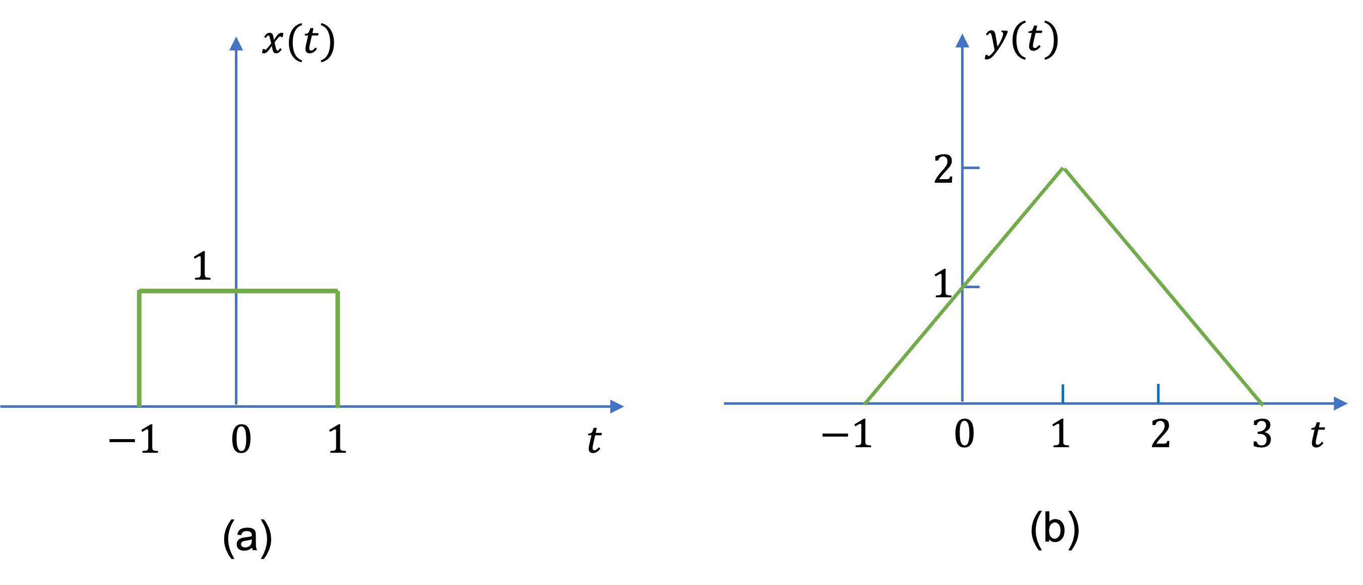
Fig. 35 Input and output signals for a continuous-time LTI system#
Sketch the output to the following inputs:
(a)\(x(t-2)\);
(b) \(\frac{1}{2}x(t)\).
For the answer, refer to the lecture recording or see solved problem 2.9 in in [Hsu, 2020].
Exercise 6.2#
Consider a continuous-time LTI system whose step response is given by
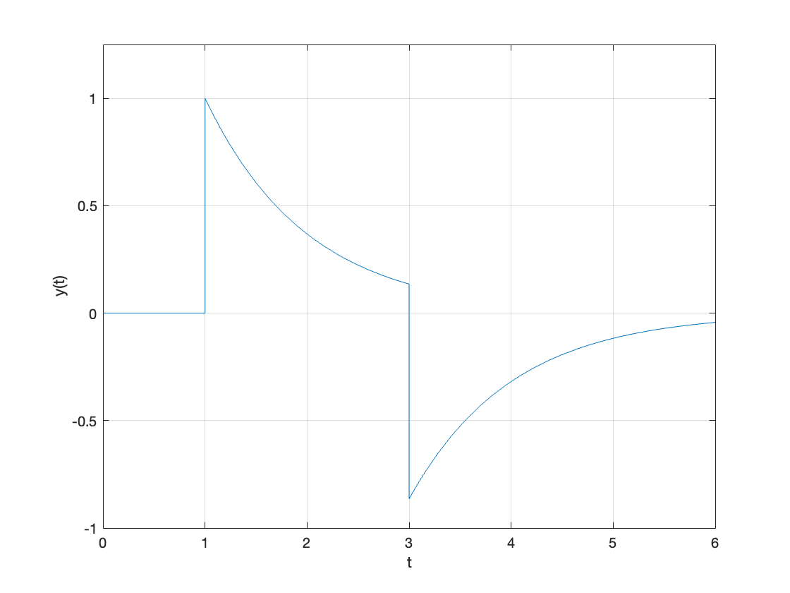
Determine and sketch the output of the system to the input \(x(t)\) shown in Fig. 36.
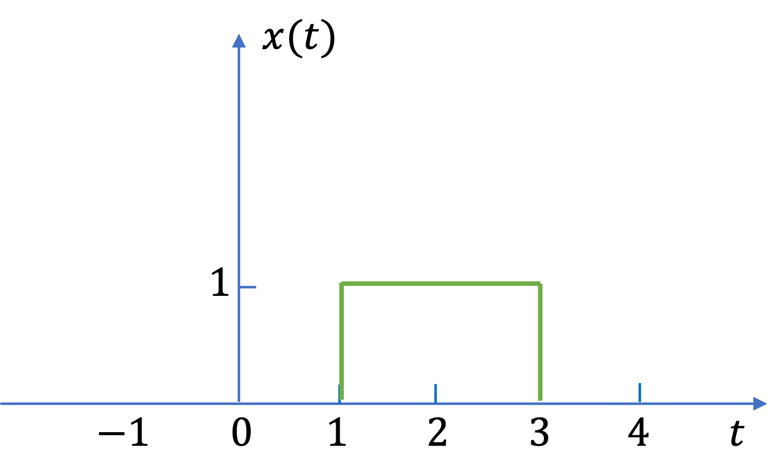
Fig. 36 Signal for Exercise 6.2#
For the answer, refer to the lecture recording or see solved problem 2.2 in in {cite}schaum.
syms t y(t)
u_0(t) = heaviside(t);
y(t) = exp(-(t-1))*u_0(t-1) - exp(-(t-3))*u_0(t-3);
fplot(y(t),[0, 6]),ylim([-1,1.25]),grid,xlabel('t'),ylabel('y(t)')
Exercise 6.3#
Note
Interesting result but not examined further.
Consider a continuous-time LTI system system described by
(a) Find and sketch the impulse response \(h(t)\) of the system.
(b) Is this system causal?
For the answer, see the solved problem 2.11 in in [Hsu, 2020].
Exercise 6.4#
Note
Interesting result but not examined further.
Let \(y(t)\) be the output of a continuous-time LTI system with input \(x(t)\). Find the output of the system if ths input is \(x'(t)\), where \(x'(t)\) is the first derivative of \(x(t)\).
For the answer, refer to the solved problem 2.12 in in [Hsu, 2020].
Exercise 6.5#
Note
Interesting result but not examined further.
Verify the BIBO stability condition (C. Stability) for continuous-time LTI systems.
For the answer, see the solved problem 2.13 in [Hsu, 2020].
Exercise 6.6#
The system shown in Fig. 37(a) is formed by connecting two systems in cascade. The impulse responses of the two systems are \(h_1(t)\) and \(h_2(t)\), respectively, and
(a) Find the impulse response \(h(t)\) of the overall system shown in Fig. 36(b).
(b) Determine if the overall system is BIBO stable.
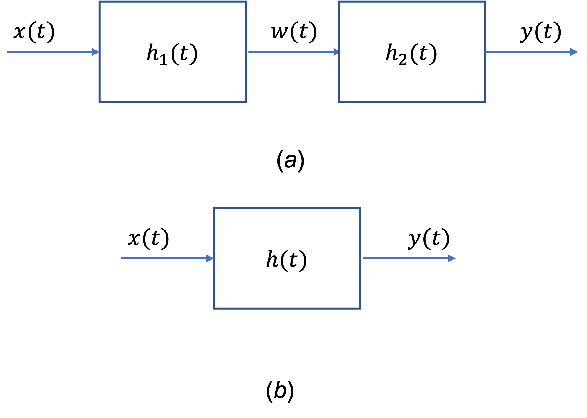
Fig. 37 A cascade connection of two continuous-time LTI systems#
For the answer, refer to the lecture recording or see solved problem 2.14 in [Hsu, 2020].
Exercises 7: Eigenfunctions of Continuous-Time LTI systems#
Exercise 7.1#
Note
This is a foretaste of the Laplace Transform.
Consider a continuous-time LTI system with the input-output relation given by
(a) Find the impulse response \(h(t)\) of this system.
(b) Show that the complex exponential \(e^{st}\) is an eigenfunction of the system.
(c) Find the eigenvalue of the system corresponding to \(e^{st}\) using the impulse response \(h(t)\) obtained in part (a).
For the answer, refer to the lecture recording or see solved problem 2.15 in [Hsu, 2020].
Exercise 7.2#
Note
Interesting result which will not be examined.
Consider the continuous-time LTI system described by
(a) Find the eigenvalue of the system corresponding to the eigenfunction \(e^{st}\).
(b) Repeat part (a) by using the impulse response \(h(t)\) of the system.
For the answer, see the solved problem 2.16 in [Hsu, 2020].
Exercise 7.3#
Note
Interesting result that is a foretaste of the Fourier transform which will not be examined.
Consider a stable continuous-time LTI system with impulse response \(h(t)\) that is real and even. Show that \(\cos \omega t\) and \(\sin \omega t\) are eigenfunctions of this system with the same eigenvalue.
For the answer, see the solved problem 2.17 in [Hsu, 2020].
Summary#
We have continued our introdiuction the continuous-time LTI systems by considering
Unit 3.2: Take aways#
Properties of continuous-time LTI systems#
The input to an LTI system is \(x(t)\), the impulse response of the LTI system is \(h(t)\) and the output is \(y(t)\).
The output of any LTI system is computed from the convolution of \(h(t)\) with \(x(t)\):
The only LTI system that has no memory is the simple gain \(y(t) = Kx(t)\) for which the impulse response \(h(t) = K\delta(t)\).
Causal LTI systems have an impulse response \(h(t)\) that satisfies \(h(t) = 0\) \(t < 0\). Therefore, for a causal LTI system the output is given by the convolution integral with adjsuted limits:
An LTI system is BIBO stable if it’s impulse response is integrable. That is:
Linear systems in series can be combined by convolution.
Eignenfunctions of continuous-time LTI systems#
The exponential signal \(x(t) = e^{st}\) (where \(s\) is a complex variable, \(s = \sigma + j\omega\)) is an eigenfunction of a continuous-time LTI system with impulse response \(h(t)\). The eigenvalue of the system is
From the equation \(y(t) = H(s)e^{st}\), \(H(s) = y(0)\).
As we will see in Unit 4.1: The Laplace Transformation, \(H(s)\) is called the Laplace transform of \(h(t)\). It is also known as the transfer function of the continuous-time LTI system that has impulse response \(h(t)\).
By a similar argument, we can show that if \(s = j\omega\), then \(e^{j\omega}\) is also an eigenfunction of \(h(t)\), and the frequency response of an LTI system is
This is called the Fourier transform and we will return to it in EG-247 Digital Signal Processing.
Next Time#
We will conclude our look at continuous-time LTI systems by considering