Unit 2.2: Periodic, Energy and Power Signals#
We continue with our survey of Signals and Classification of Signals by looking at Periodic and Nonperiodic Signals and Energy and Power Signals.
This section is based on Section 1.2 of [Hsu, 2020].
Follow along at cpjobling.github.io/eg-150-textbook/signals_and_systems/signals/pep_signals

Periodic and Nonperiodic Signals#
Periodic signals#
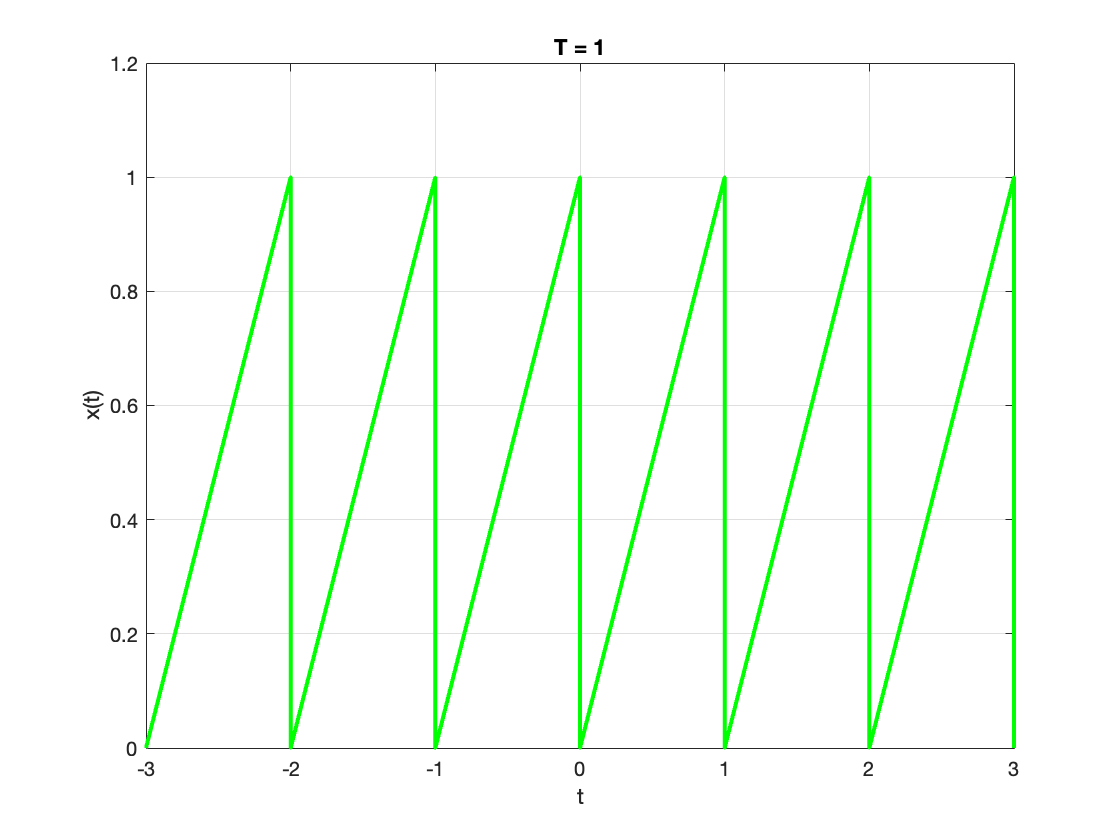
A continuous-time signal \(x(t)\) is said to be periodic with period \(T\) if there is a positive nonzero value of \(T\) for which
An example of such a signal is given in Fig. 17.
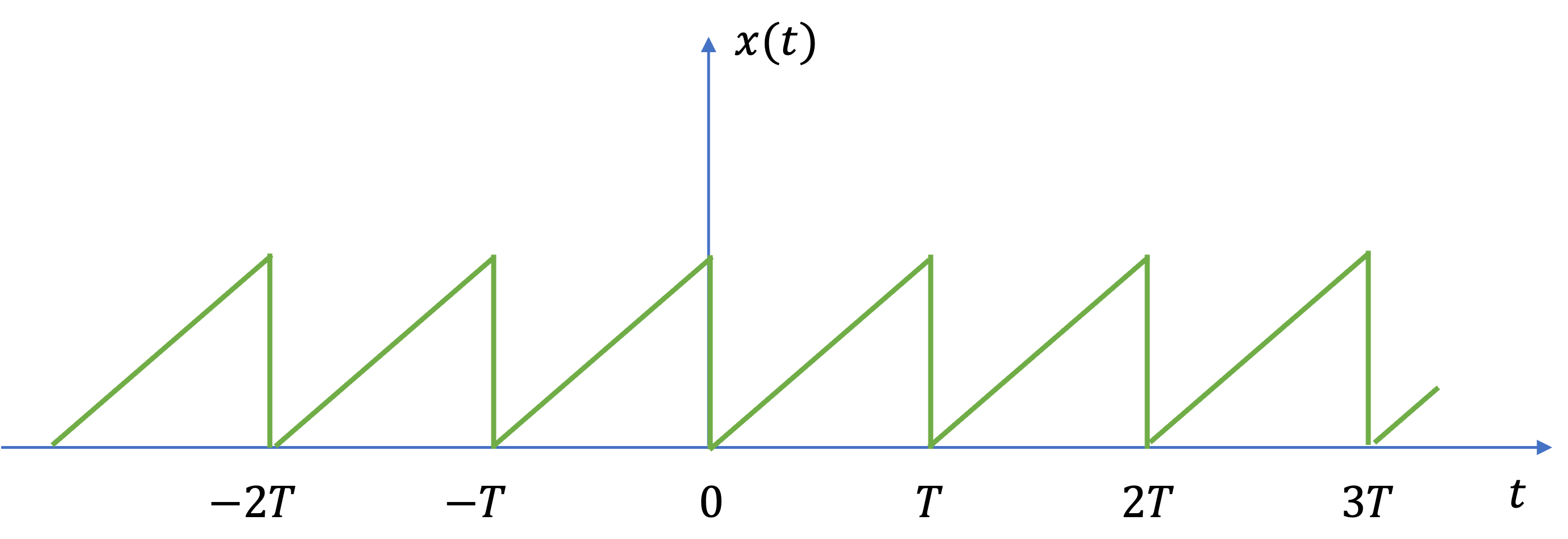
Fig. 17 An example of a periodic signal.#
We can use the periodicity to synthesize a periodic signal such as that shown in Fig. 17.
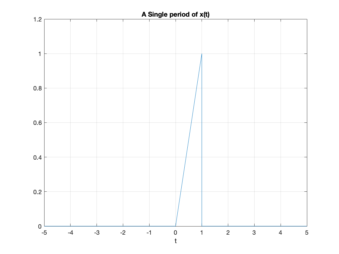
Let’s first define the signal over one period. We will use MATLAB and the symbolic math toolbox for this example:
Let one period of the periodic signal be defined by
We can use the Heaviside function (unit step) (MATLAB function heaviside: see The Unit Step Function) to sythesise this signal.
Define a \(t\) as a symbolic variable t
syms t
Define the period \(T\) of the periodic signal (you might want to play with this value)
T = 1; % period of periodic signal
Now define the signal using the Heaviside function to limit the range of the signal.
x(t) = t * (heaviside(t) - heaviside(t-T));
Now plot one period of the signal \(x(t)\)
fplot(x(t)),ylim([0 1.2]),grid,title('A Single period of x(t)'),xlabel('t')
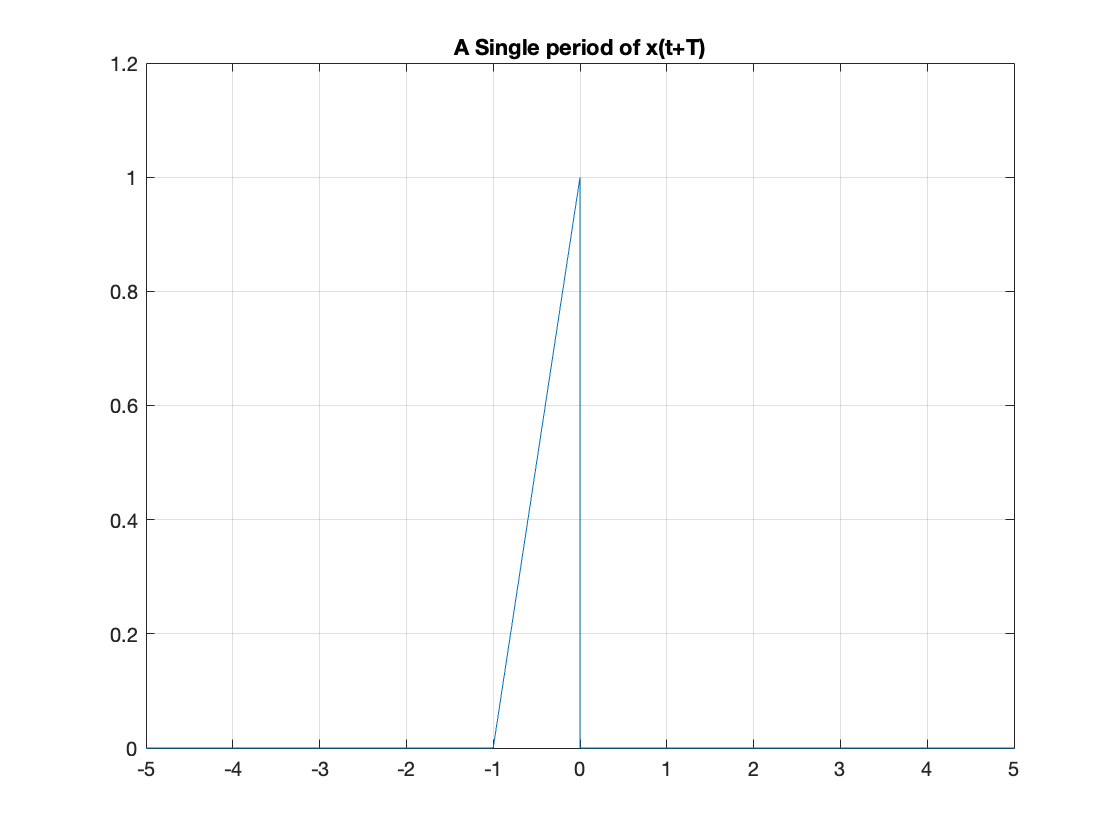
One period earlier:
signal1 = x(t + T)
fplot(signal1),ylim([0 1.2]),grid,title('A Single period of x(t+T)')
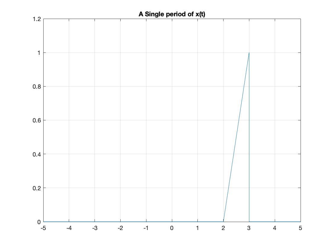
Two periods later:
signal2 = x(t-2*T)
fplot(signal2),ylim([0 1.2]),grid,title('A Single period of x(t)')
It follows that
for all \(t\) and any integer \(m\).
Now we use a loop and the definition of periodic function to repeat this signal multiple times
periodic_signal = 0;
for m = 5:-1:-5
    periodic_signal = periodic_signal + x(t + m*T);
end
periodic_signal
Now we plot the result
fplot(periodic_signal,'g-',"LineWidth",2),...
    grid,ylabel('x(t)'),xlabel('t'),title('T = 1')
xlim([-3.00 3.00])
ylim([0 1.2])
Fundamental period#
The fundamental period \(T_0\) of \(x(t)\) is the smallest value of \(T\) for which \(x(t + mT) = x(t)\) holds.
For the previous example this was \(T_0=1\).
DC signals#
Note that the definition of the fundamental period does not hold for a constant signal \(x(t)\) (known as a DC signal).
For a constant signal \(x(t) = c\) the fundamental period is undefined since \(x(t)\) is periodic for any choice of \(T\) (and so there is no smallest postive value). See Fig. 18.
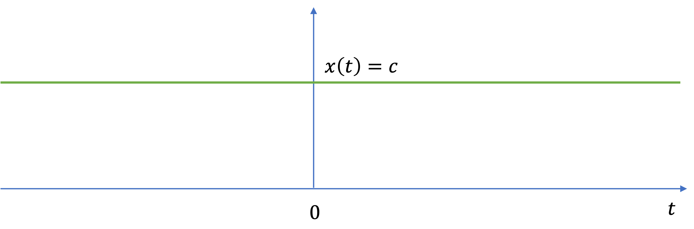
Fig. 18 A DC signal#
Note
Note that the sum of two continuous time signals may not be periodic (Example Example 2.1: Sum of two periodic signals)
Nonperiodic signals#
Any continuous-time signal which is not periodic is called a nonperiodic (or aperiodic) signal. For example see Fig. 19
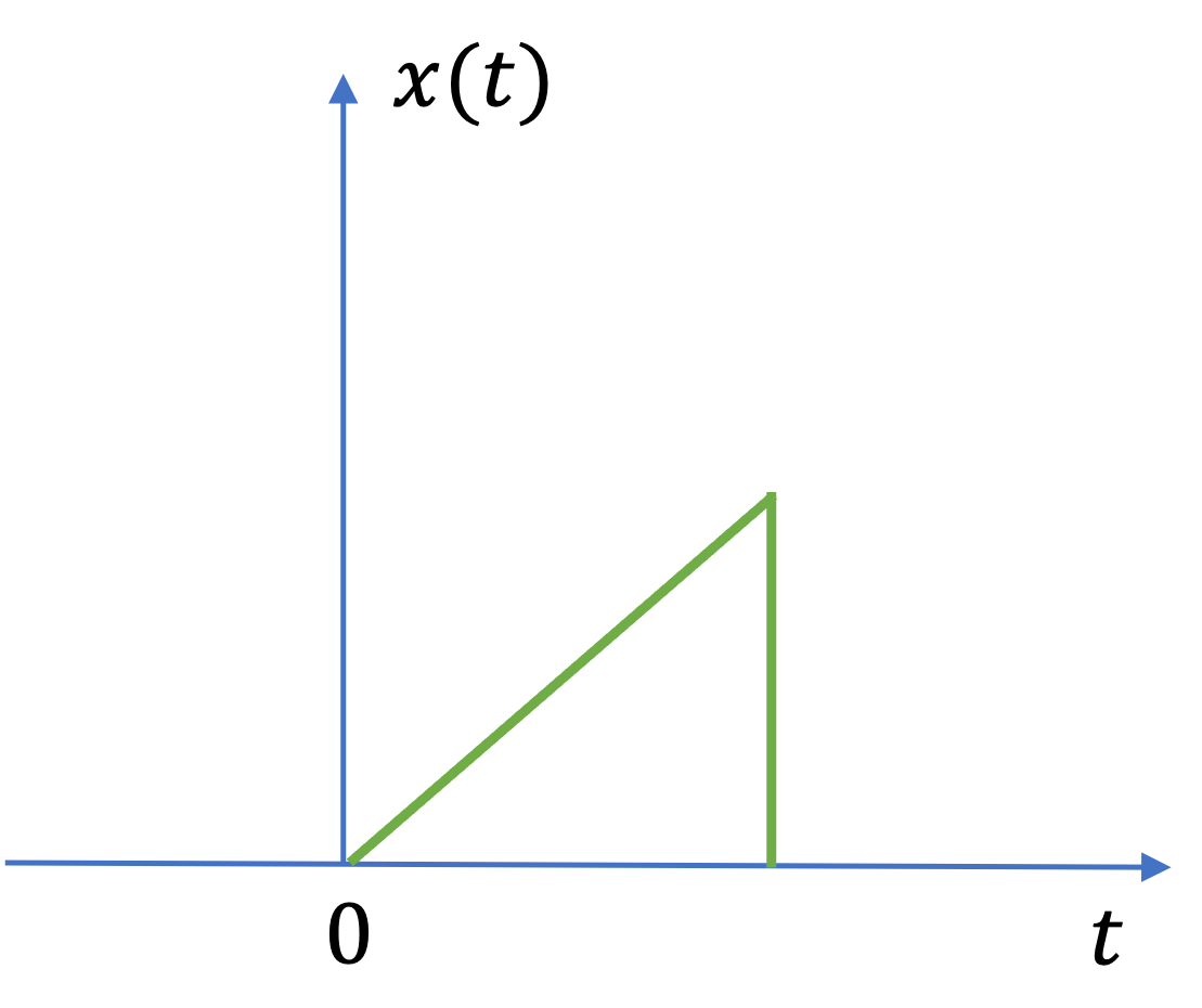
Fig. 19 A nonperiodic signal#
Energy and Power Signals#
Consider \(v(t)\) to be the voltage across a resistor \(R\) producing a current \(i(t)\). (Fig. 20)
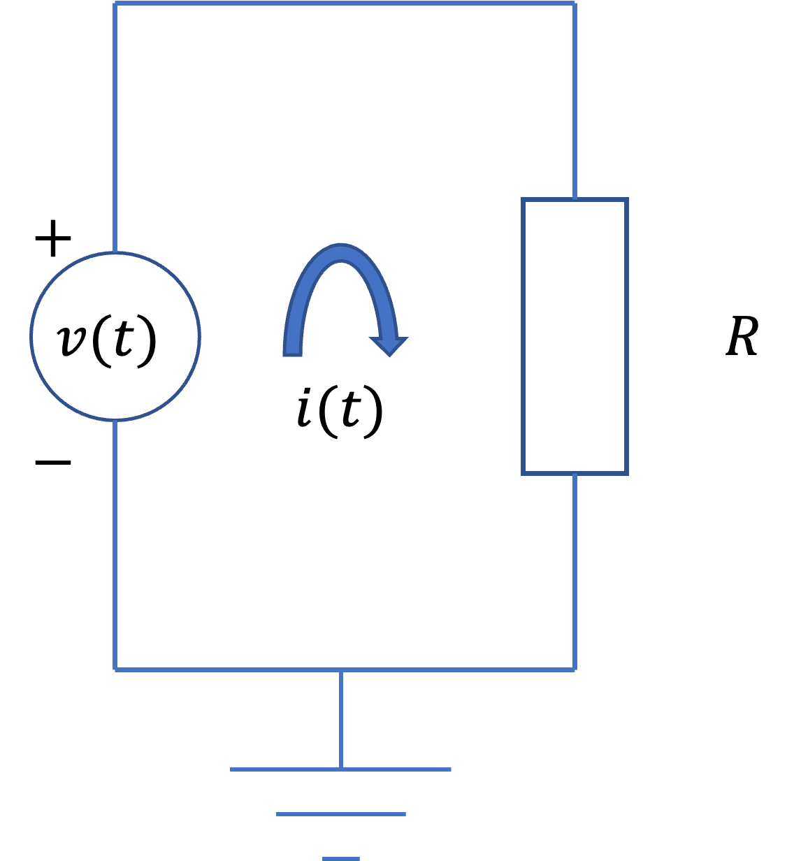
Fig. 20 A simple resistor circuit.#
The instantaneous power \(p(t)\) per ohm is defined as
Total energy \(E\) and average power \(P\) on a per-ohm basis are
Normalised energy content of a signal#
For an arbitrary continuous-time signal \(x(t)\), the normalised energy content \(E\) of \(x(t)\) is defined as
Normalised average power of a signal#
The normalised average power \(P\) of \(x(t)\) is defined as
Energy and power signals#
Based on the previous definitions, the following classes of signals can be defined:
\(x(t)\) is said to be an energy signal if and only if \(0 < E < \infty\), and so \(P = 0\).
\(x(t)\) is said to be an power signal if and only if \(0 < P < \infty\), thus implying that \(E = \infty\).
Signals that satisfy neither property are referred to as neither energy signals nor power signals.
Note that a periodic signal is a power signal if its energy content per period is finite, and then the average power of this signal need only be calulated over a period (ex:1.18).
Other Measures of Signal Size#
There are other measures of signal size that are used:
Mean value#
For periodic signals with fundamental period \(T_0\)
The mean value is also known as the dc value.
Observations
the mean value corresponds to the arithmetic average
the signal \(x(t) - M_x\) has zero mean
Measures of spread#
Root-mean square (RMS)#
E.g. the power of \(x(t) = A\sin\left(\omega t + \theta\right)\) is \(A^2/2\) hence its RMS value is \(A/\sqrt{2}\).
Peak value#
Crest factor (CF)#
Peak-to-average power ratio (PAPR)#
Observations
CF and PAPR measure the dispersion of a signal about its average power.
To express CF or PAPR we often use decibels (dB). To obtain a measure of the quantity \(y\) in dB use \(20\log_{10}(y)\).
Exercises 2#
Example 2.1: Sum of two periodic signals#
Let \(x_1(t)\) and \(x_2(t)\) be periodic signals with fundamental periods \(T_1\) and \(T_2\) respectively. Under which conditions is the sum \(x(t) = x_1(t) + x_2(t)\) periodic, and what is the fundamental period of \(x(t)\) if it is periodic?
For the answer, refer to the lecture recording or see solved problem 1.14 in [Hsu, 2020].
Exercise 2.2: Periodic signals#
MATLAB Example
We will solve this example by hand and then give the solution in the MATLAB lab.
Determine whether or not each of the following signals is periodic. If a signal is periodic, determine its fundamental period.
a). \(x(t)=\cos\left(t + \frac{\pi}{4}\right)\);
b). \(x(t)=\sin\frac{2\pi}{3}t\);
c). \(x(t)=\cos\frac{\pi}{3}t+\sin\frac{\pi}{4}t\);
d). \(x(t)=\cos t + \sin\sqrt{2}t\);
e). \(x(t)=\sin^2t\);
f). \(x(t)=e^{j\left[(\pi/2)t-1\right]}\);
For the answers, refer to the lecture recording or see solved problem 1.16 in [Hsu, 2020].
Exercise 2.3: Integral properties of periodic signals#
Show that if \(x(t + T) = x(t)\), then
for any real \(\alpha\), \(\beta\) and \(a\).
For the answer, refer to the lecture recording or see solved problem 1.17 in [Hsu, 2020].
Exercise 2.4: Power in a periodic signal#
Show that if \(x(t)\) is periodic with fundamental period \(T_0\), then the normalized average power \(P\) of \(x(t)\) defined by
is the same as the average power \(x(t)\) over any interval of length \(T_0\), that is,
For the answer, refer to the lecture recording or see solved problem 1.18 in [Hsu, 2020].
Exercise 2.5: Power and energy signals#
MATLAB Example
We will solve this example by hand and then give the solution in the MATLAB lab.
Determine whether the following signals are energy signals, power signals, or neither.
a). \(x(t)=e^{-at}u_0(t)\), \(a > 0\);
b). \(x(t)=A\cos\left(\omega_0 t + \theta\right)\)
c). \(x(t)=t u_0(t)\)
Note \(u_0(t)\) is the unit step (or Heaviside) function formally introduced in the next lecture. For the answer, refer to the lecture recording or see solved problem 1.20 in [Hsu, 2020].
Exercise 2.6: Power in domestic mains electricty#
Domestic mains power in the UK is delivered as a sinusoidal signal \(x(t)=A\cos(\omega_0 t + \theta)\) with frequency of \(50\mathrm{Hz}\) and RMS value of \(240\mathrm{V}\).
Calculate the fundamental period \(T_0\), fundamental angular frequency \(\omega_0\), average power \(P\), peak voltage \(A = x_\mathrm{peak}\), crest factor (CF) and peak-to-average power ratio (PAPR) of the power signal provided to the home.
Express CF and PAPR in dB.
Summary#
In this lecture we completed our look at signals and the classification of signals.
In particular we have looked at
Energy and Power Signals of a signal \(x(t)\)
Unit 2.2: Take aways#
A signal is periodic, with period \(T\) is \(x(t + T) = x(t)\;\mathrm{all}\;t\)
Signal energy for a signal \(x(t)\):
Signal power for a signal \(x(t)\):
\(x(t)\) is said to be an energy signal if and only if \(0 < E < \infty\), and so \(P = 0\).
\(x(t)\) is said to be an power signal if and only if \(0 < P < \infty\), thus implying that \(E = \infty\).
Signals that satisfy neither property are referred to as neither energy signals nor power signals.
Signal mean (average or DC value):
Root mean square (RMS): \(\sqrt{P_x}\);
Peak value: \(\left|x\right|_\mathrm{peak} = \max_t \left|x(t)\right|\);
Crest factor:
Peak-to-average power ratio (PAPR):
Value of \(y\) in decibel (dB) is \(20\log_{10} y\).