Unit 4.4 The Inverse Laplace Transform

Unit 4.4 The Inverse Laplace Transform#

Follow along at cpjobling.github.io/eg-150-textbook/laplace_transform/4/inverse_laplace

QR Code for this lecture

Introduction#

The preparatory reading for this section is Chapter 3 of [Karris, 2012] which

defines the Inverse Laplace transformation
gives several examples of how the Inverse Laplace Transform may be obtained
thouroughly decribes the Partial Fraction Expansion method of converting complex rational polymial expressions into simple first-order and quadratic terms
demonstrates the use of MATLAB for finding the poles and residues of a rational polymial in s and the symbolic inverse laplace transform.

There is additional coverage, including many worked problems in Chapter 3.5 of [Hsu, 2020].

We will explore the use of MATLAB to solve inverse Laplace tranforms in MATLAB Lab 4.

Agenda#

Definition
Partial Fraction Expansion
Inverse Laplace Transform by Partial Fraction Expansion (PFE)
Exercises 11: Inverse Laplace Transforms

Definition#

The formal definition of the inverse Laplace transform is

(2)#

L^{- 1} {F (s)} = \frac{1}{2 π j} \int_{σ - j ω}^{σ + j ω} F (s) e^{s t} d s

but this is difficult to use in practice because it requires contour integration using complex variable theory.

For most engineering problems we can instead refer to Tables of Properties and Common Transform Pairs to look up the Inverse Laplace Transform.

(Or, if we are not taking an exam, we can use a computer or mobile device.)

Partial Fraction Expansion#

Quite often the Laplace Transform we start off with is a rational polynomial in $s$ .

(3)#

F (s) = \frac{N (s)}{D (s)} = \frac{b_{m} s^{m} + b_{m - 1} s^{m - 1} + b_{m - 2} s^{m - 2} + \dots + b_{1} s + b_{0}}{a_{n} s^{n} + a_{n - 1} s^{n - 1} + a_{n - 2} s^{n - 2} + \dots + a_{1} s + a_{0}}

The coefficients $a_{n}$ and $b_{n}$ are real for $n = 1, 2, 3, \dots$

Proper and Improper Rational Functions#

If $m < n$ $F (s)$ is said to be a proper rational function.
If $m \geq n$ $F (s)$ is said to be an improper rational function

(Think proper fractions and improper fractions.)

Zeros#

The roots of the numerator polymonial $N (s)$ are found by setting $N (s) = 0$
When $s$ equals one of the $m$ roots of $N (s)$ then $F (s)$ will be zero.
Thus the roots of $N (s)$ are the zeros of $F (s)$ .

Poles#

The roots (zeros) of the denominator polynomial are found by setting $D (s) = 0$ .
When $s$ equals one of the $n$ roots of $D (s)$ then $F (s)$ will be infinite $F (s_{r}) = N (s_{r}) / 0 = \infty$ ).
These are called the poles of $F (s)$ .

(Imagine telegraph poles planted at the points on the $s$ -plane where $D (s)$ is zero.)

A Further Simplifying Assumption#

If $F (s)$ is proper then it is conventional to make the coefficient $s_{n}$ unity thus:

(4)#

F (s) = \frac{N (s)}{D (s)} = \frac{1 / a_{n} (b_{m} s^{m} + b_{m - 1} s^{m - 1} + b_{m - 2} s^{m - 2} + \dots + b_{1} s + b_{0})}{s^{n} + \frac{a_{n - 1}}{a_{n}} s^{n - 1} + \frac{a_{n - 2}}{a_{n}} s^{n - 2} + \dots + \frac{a_{1}}{a_{n}} s + \frac{a_{0}}{a_{n}}}

(I know it doesn’t look simpler, but remember that the $a$ and $b$ coefficients are numbers in practice!)

Inverse Laplace Transform by Partial Fraction Expansion (PFE)#

The poles of $F (s)$ can be real and distinct, real and repeated, complex conjugate pairs, or a combination.

Defining the problem#

The nature of the poles governs the best way to tackle the PFE that leads to the solution of the Inverse Laplace Transform. Thus, we need to structure our presentation to cover one of the following cases:

The case where $F (s)$ has distinct real poles
The case where $F (s)$ has complex poles
The case where $F (s)$ has repeated poles
The case where $F (s)$ is an improper rational polynomial

We will examine each case by means of a worked example. Please refer to Chapter 3 of Karris for full details.

The case of the distinct real poles#

If the poles $p_{1}, p_{2}, p_{3}, \dots, p_{n}$ are distinct we can factor the denominator of $F (s)$ in the form

(5)#

F (s) = \frac{N (s)}{(s - p_{1}) (s - p_{2}) (s - p_{3}) \dots (s - p_{n})}

Next, using partial fraction expansion

(6)#

F (s) = \frac{r_{1}}{s - p_{1}} + \frac{r_{2}}{s - p_{2}} + \frac{r_{3}}{s - p_{3}} + \dots + \frac{r_{n}}{s - p_{n}}

To evaluate the residue $r_{k}$ , we multiply both sides by $(s - p_{k})$ then let $s \to p_{k}$

(7)#

r_{k} = lim_{s \to p_{k}} (s - p_{k}) F (s) = {(s - p_{k}) F (s) |}_{s = p_{k}}

The case of the complex poles#

Quite often the poles of $F (s)$ are complex and because the complex poles occur as complex conjugate pairs, the number of complex poles is even. Thus if $p_{k}$ is a complex root of $D (s)$ then its complex conjugate $p_{k}^{*}$ is also a root of $D (s)$ .

You can still use the PFE with complex poles, as demonstrated in Pages 3-5—3-7 in the textbook. However it is easier to use the fact that complex poles will appear as quadratic factors of the form $s^{2} + a s + b$ and then call on the two transforms in the PFE

(8)#

\frac{ω}{(s - a)^{2} + ω^{2}} \Leftrightarrow e^{a t} \sin ω t

(9)#

\frac{s + a}{(s - a)^{2} + ω^{2}} \Leftrightarrow e^{a t} \cos ω t

The case of the repeated poles#

When a rational polynomial has repeated poles

(10)#

F (s) = \frac{N (s)}{(s - p_{1})^{m} (s - p_{2}) \dots (s - p_{n - 1}) (s - p_{0})}

and the PFE will have the form:

\begin{array}{r} \begin{array}{c} F (s) = \frac{r_{11}}{(s - p_{1})^{m}} + \frac{r_{12}}{(s - p_{1})^{m - 1}} + \frac{r_{13}}{(s - p_{1})^{m - 2}} + \dots + \frac{r_{1}}{(s - p_{1})} \\ + \frac{r_{2}}{(s - p_{2})} + \frac{r_{3}}{(s - p_{3})} + \dots + \frac{r_{n}}{(s - p_{n})} \end{array} \end{array}

The ordinary residues $r_{k}$ can be found using the rule used for distinct roots.

To find the residuals for the repeated term $r_{1 k}$ we need to multiply both sides of the expression by $(s + p_{1})^{m}$ and take repeated derivatives as described in detail in Pages 3-7—3-9 of the text book. This yields the general formula

(11)#

r_{1 k} = lim_{s \to p_{1}} \frac{1}{(k - 1)!} \frac{d^{k - 1}}{d s^{k - 1}} [(s - p_{1})^{m} F (s)]

which in the age of computers is rarely needed.

The case of the improper rational polynomial#

If $F (s)$ is an improper rational polynomial, that is $m \geq n$ , we must first divide the numerator $N (s)$ by the denomonator $D (s)$ to derive an expression of the form

(12)#

F (s) = k_{0} + k_{1} s + k_{2} s^{2} + \dots + k_{m - n} s^{m - n} + \frac{N (s)}{D (s)}

and then $N (s) / D (s)$ will be a proper rational polynomial.

Exercises 11: Inverse Laplace Transforms#

Lecturer clear all cells and set up MATLAB

clear all
% setappdata(0, "MKernel_plot_format", 'svg')
format compact

Starting MATLAB ...

Error connecting to MATLAB. Check the status of MATLAB by clicking the "Open MATLAB" button. Retry after ensuring MATLAB is running successfully

Exercise 11.1: Real Poles#

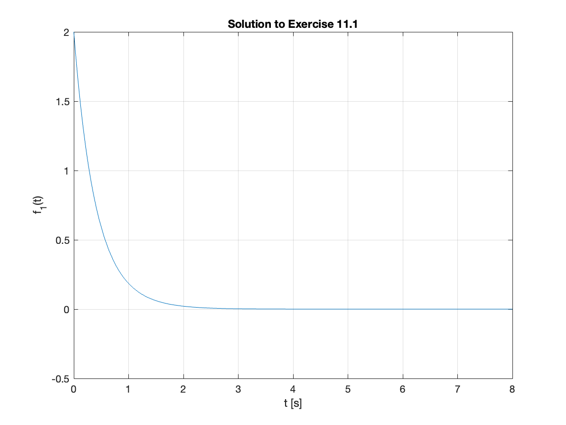
Use the PFE method to simplify $F_{1} (s)$ below and find the time domain function $f_{1} (t)$ corresponding to $F_{1} (s)$

F_{1} (s) = \frac{2 s + 5}{s^{2} + 5 s + 6}

(Quick solution: Wolfram Alpha)

Paper Solution#

See OneNote class notebook: Unit 4.4: The Inverse Transform.

MATLAB Solution - Numerical#

Ns = [2, 5]; Ds = [1, 5, 6];
[r,p,k] = residue(Ns, Ds)

Error connecting to MATLAB. Check the status of MATLAB by clicking the "Open MATLAB" button. Retry after ensuring MATLAB is running successfully

This result should be interpreted as:

F_{1} (s) = \frac{1}{s + 3} + \frac{1}{s + 2}

which because of the linearity property of the Laplace Transform and using tables results in the Inverse Laplace Transform

f_{1} (t) = e^{- 3 t} u_{0} (t) + e^{- 2 t} u_{0} (t)

MATLAB solution - symbolic#

Recall that in MATLAB the laplace operator is the single sided Laplace transform, so the presence of $u_{0} (t)$ in the answers given by ilaplace is implied.

syms s t;
F_1(s) = (2*s + 5)/(s^2 + 5*s + 6);
f_1(t) = ilaplace(F_1(s))

Error connecting to MATLAB. Check the status of MATLAB by clicking the "Open MATLAB" button. Retry after ensuring MATLAB is running successfully

Which we can plot using the fplot function:

fplot(f_1(t),[0,8]),title('Solution to Exercise 11.1'),ylim([-0.5,2.0]),grid,ylabel('f_1(t)'),xlabel('t [s]')

Error connecting to MATLAB. Check the status of MATLAB by clicking the "Open MATLAB" button. Retry after ensuring MATLAB is running successfully

Exercise 11.2: Cubic with Real Poles#

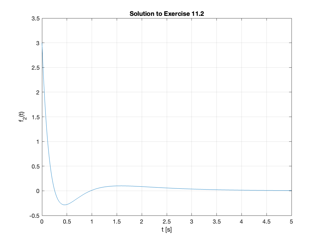
Determine the Inverse Laplace Transform of

F_{2} (s) = \frac{3 s^{2} + 2 s + 5}{s^{3} + 9 s^{2} + 23 s + 15}

(Quick solution: Wolfram Alpha)

Solution 11.2#

Because the denominator of $F_{2} (s)$ is a cubic, it will be difficult to factorise without computer assistance so we use MATLAB to factorise $D (s)$

syms s;
factors = factor(s^3 + 9*s^2 + 23*s + 15)

Error connecting to MATLAB. Check the status of MATLAB by clicking the "Open MATLAB" button. Retry after ensuring MATLAB is running successfully

In an exam you’d be given the factors

The problem becomes: determine the Inverse Laplace Transform of

F_{2} (s) = \frac{3 s^{2} + 2 s + 5}{(s + 1) (s + 3) (s + 5)}

which we will solve in class.

Paper Solution#

See OneNote class notebook: Unit 4.4: The Inverse Transform.

The solution checked with MATLAB should be

f_{1} (t) = \frac{3}{4} e^{- t} - \frac{13}{2} e^{- 3 t} + \frac{35}{4} e^{- 5 t}

Symbolic Solution#

F_2(s) = (3*s^2 + 2*s + 5)/((s+1)*(s+3)*(s+5))
f_2(t) = ilaplace(F_2(s))

Error connecting to MATLAB. Check the status of MATLAB by clicking the "Open MATLAB" button. Retry after ensuring MATLAB is running successfully

Which can be plotted using fplot. Note that it is good practice to adjust the scale and label your plots.

fplot(f_2(t),[0,5]),ylim([-0.5,3.5]),grid,title('Solution to Exercise 11.2'),ylabel('f_2(t)'),xlabel('t [s]')

Error connecting to MATLAB. Check the status of MATLAB by clicking the "Open MATLAB" button. Retry after ensuring MATLAB is running successfully

Exercise 11.3: System with Complex Poles#

Rework Example 3-2 from the [Karris, 2012] using quadratic factors.

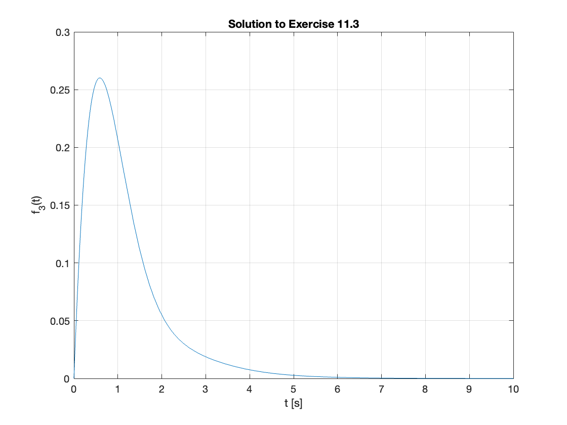
Find the Inverse Laplace Transform of

(13)#

F_{3} (s) = \frac{s + 3}{(s + 1) (s^{2} + 4 s + 8)}

(Quick solution: Wolfram Alpha – Shows that the computer will not always give the expected answer!)

Solution 11.3#

We know that one pole is real at $s = - 1$ . We can use the PFE in the usual way to find the residue $r_{1}$ that corresponds to that pole.

We can use residue to find the other two poles, but the poles and the residues will both be complex:

Ns = [1 3]; Ds = conv([1 1],[1 4 8]) % conv of two vectors is polynomial multiplication
[r,p,k]=residue(Ns,Ds)

Error connecting to MATLAB. Check the status of MATLAB by clicking the "Open MATLAB" button. Retry after ensuring MATLAB is running successfully

We can use PFE to solve this, as is done in Section 3.2.2 of [], but the mathematics is quite challenging.

Instead, we assume that the solution will have the structure

F_{3} (s) = \frac{2 / 5}{s + 1} + r_{2} \frac{ω}{(s + a)^{2} + ω^{2}} + r_{3} \frac{s + a}{(s + a)^{2} + ω^{2}}

and solve the PFE using simultaneous equations to determine $r_{2}$ and $r_{3}$ .

Complete the square on the quadratic term:

s^{2} + 4 s + 8 = (s + 2)^{2} + 4

Then comparing this with the desired form $(s + a)^{2} + ω^{2}$ , we have $a = 2$ and $ω^{2} = 4 \to ω = \sqrt{4} = 2$ .

To solve this, we need to find the PFE for the assumed solution:

(14)#

F_{3} (s) = \frac{2 / 5}{s + 1} + r_{2} \frac{2}{(s + 2)^{2} + 2^{2}} + r_{3} \frac{s + 2}{(s + 2)^{2} + 2^{2}}

which we do by equating (14) to (13),

(15)#

\frac{s + 3}{(s + 1) (s^{2} + 4 s + 8)} = \frac{2 / 5}{s + 1} + r_{2} \frac{2}{(s + 2)^{2} + 2^{2}} + r_{3} \frac{s + 2}{(s + 2)^{2} + 2^{2}}

putting both sides on a common denominator,

(16)#

\frac{s + 3}{(s + 1) (s^{2} + 4 s + 8)} = \frac{(2 / 5) (s^{2} + 4 s + 8) + r_{2} (s + 1) + r_{3} (s + 1) (s + 2)}{(s + 1) (s^{2} + 4 s + 8)}

and then solving for $r_{2}$ and $r_{3}$ by equating the numerator coefficients on the left and right sides.

s + 3 = (2 / 5) (s^{2} + 4 s + 8) + r_{2} (s + 1) + r_{3} (s^{2} + 3 s + 2)

The completion of this problem is left as a homework exercise for the student.

The solution should be:

(17)#

f_{3} (t) = \frac{2}{5} e^{- t} + \frac{3}{10} e^{- 2 t} \sin 2 t - \frac{2}{5} e^{- 2 t} \cos 2 t

You can use trig. identities to simplify this further if you wish.

Symbolic solution#

F_3(s) = (s+3)/((s+1)*(s^2 + 4*s + 8))
f_3(t) = ilaplace(F_3(s))
fplot(f_3(t),[0,10]),ylim([0,0.3]),grid,title('Solution to Exercise 11.3'),ylabel('f_3(t)'),xlabel('t [s]')

Error connecting to MATLAB. Check the status of MATLAB by clicking the "Open MATLAB" button. Retry after ensuring MATLAB is running successfully

Exercise 11.4: Repeated Real Poles#

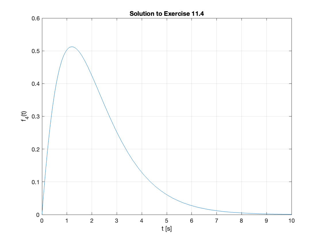
Find the inverse Laplace Transform of

F_{4} (s) = \frac{s + 3}{(s + 2) (s + 1)^{2}}

Note that the transform

t e^{a t} \Leftrightarrow \frac{1}{(s - a)^{2}}

and the derivative of a quotient rule

\frac{d}{d s} (\frac{N (s)}{D (s)}) = \frac{D (s) \frac{d N (s)}{d s} - N (s) \frac{d D (s)}{d s}}{D (s)^{2}}

will be useful.

(Quick solution: Wolfram Alpha)

Solution 11.4#

We will leave the solution that makes use of the residude of repeated poles formula for you to study from the text book (Example 3.4 []).

In class we will illustrate the slightly simpler approach also presented in the text.

For exam preparation, I would recommend that you use whatever method you find most comfortable.

Find the inverse Laplace Transform of

F_{4} (s) = \frac{s + 3}{(s + 2) (s + 1)^{2}}

Symbolic solution#

F_4(s) = (s + 3)/((s+2)*(s+1)^2)
f_4(t) = ilaplace(F_4(s))
fplot(f_4(t),[0,10]),grid,ylim([0,0.6]),title('Solution to Exercise 11.4'),ylabel('f_4(t)'),xlabel('t [s]')

Error connecting to MATLAB. Check the status of MATLAB by clicking the "Open MATLAB" button. Retry after ensuring MATLAB is running successfully

Numerical solution#

We use function conv to perform polynomial multiplication

Ns = [1 3]
Ds = conv([1 2],conv([1 1],[1 1])) % (s + 2)*(s + 1)*(s + 1)
[r,p,k] = residue(Ns,Ds)
doc residue

Error connecting to MATLAB. Check the status of MATLAB by clicking the "Open MATLAB" button. Retry after ensuring MATLAB is running successfully

To interpret this we refer to the MATLAB documentation doc residue which tells us, that for the pole at $s = - 1$ , the first residue (here $r_{2} = - 1$ ) is for the term $1 / (s + 1)$ and the second (here $r_{3} = 2$ ) is for $1 / (s + 1)^{2}$ . Thus the PFE is

F_{4} (s) = \frac{1}{s + 2} - \frac{1}{s + 1} + \frac{2}{(s + 1)^{2}}

hence

f_{4} (t) = e^{- 2 t} u_{0} (t) - e^{- t} u_{0} (t) + 2 t e^{- t} u_{0} (t)

Exercise 11.5: Non-proper rational polynomial#

Introduces some new transform pairs!

F_{6} (s) = \frac{s^{2} + 2 s + 2}{s + 1}

(Quick solution: Wolfram Alpha)

Solution 11.5#

Dividing $s^{2} + 2 s + 2$ by $s + 1$ gives

F_{6} (s) = s + 1 + \frac{1}{s + 1}

\frac{1}{s + 1} \Leftrightarrow e^{- t}

1 \Leftrightarrow δ (t)

s \Leftrightarrow ?

What function of t has Laplace transform s?#

Recall from Session 2:

\frac{d}{d t} u_{0} (t) = u_{0}^{'} (t) = δ (t)

and

\frac{d^{2}}{d t^{2}} u_{0} (t) = u_{0}^{″} (t) = δ^{'} (t)

Also, by the time differentiation property

u_{0}^{″} (t) = δ^{'} (t) \Leftrightarrow s^{2} L u_{0} (t) - s u_{0} (0^{-}) - {\frac{d}{d t} u_{0} (t) |}_{t = 0^{-}} = s^{2} \frac{1}{s} = s

New Transform Pairs#

s \Leftrightarrow δ^{'} (t)

\frac{d^{n}}{d t^{n}} δ (t) \Leftrightarrow s^{n}

f_{6} (t) = e^{- t} + δ (t) + δ^{'} (t)

Matlab verification#

Ns = [1, 2, 2]; Ds = [1 1];
[r, p, k] = residue(Ns, Ds)

Error connecting to MATLAB. Check the status of MATLAB by clicking the "Open MATLAB" button. Retry after ensuring MATLAB is running successfully

syms s;
F_6(s) = (s^2 + 2*s + 2)/(s + 1);
f_6(t) = ilaplace(F_6(s))

Error connecting to MATLAB. Check the status of MATLAB by clicking the "Open MATLAB" button. Retry after ensuring MATLAB is running successfully

Lab Work#

In MATLAB Lab 4, we will explore the tools provided by MATLAB for taking Laplace transforms, representing polynomials, finding roots and factorizing polynomials and solution of inverse Laplace transform problems.

Unit 4.4: Homework#

Complete Exercise 11.3: System with Complex Poles to confirm the result (16). Then do the end of the chapter exercises (Section 3.67) from the [Karris, 2012]. Don’t look at the answers until you have attempted the problems.

Summary#

In this section we have looked at the inverse Laplace transform. In particular, how to solve continuous-time LTI system problems that take the form of rational polynomials in $s$ .

Definition
Partial Fraction Expansion
Inverse Laplace Transform by Partial Fraction Expansion (PFE)
Exercises 11: Inverse Laplace Transforms

Unit 4.4: Take Aways#

For causal signals and continuous-time LTI systems, the Laplace transform usually takes the form of a rational polynomial with general form $F (s)$ as shown in equation (3). The denominator of $F (s)$ , $D (s)$ , can always be factorised, and the factors (zeros of D(s), poles of F(s)) will be real $(s - p_{k})$ , real and repeated, such as $(s - p_{k})^{n}$ or complex conjugate pairs $(s - σ_{k} - j ω_{k}) (s - σ_{k} + j ω_{k})^{1}$ , or a combination of these.

Each such rational polynomial can then be represented as a partial fraction with residues $r_{k}$ whose values are determined by using one of the partial fraction expansion methods presented in this unit:

The case of the distinct real poles
The case of the complex poles
The case of the repeated poles
The case of the improper rational polynomial

The factored polynomial which represents $F (s)$ can then be converted into the equivalent $f (t)$ by use of the linearity property (Linearity) and tables of Laplace transforms (e.g. ap:xform_table).

MATLAB#

The inverse Laplace transform is given by the Symbolic math toolbox function ilaplace. We can determine the partial fraction of a rational polynomial with constant coefficients using the function residue we can factorise a symbolic polynomial using factor and expand a product of rational terms using expand. A symbolic polynomial with numerical coeffients can be converted into a numerial polynomial using sym2poly and you can go the other way using poly2sym. For more information and examples on how to use these functions please consult the MATLAB help centre.

Footnote

1 A pair of complex conjugate factors

(s - σ - j ω) (s - σ + j ω)

can be represented as a single quadratic factor which, when $σ < 0$ , will be

s^{2} + 2 σ s + (σ^{2} + ω^{2})

By completing the square we get

(s + σ)^{2} - σ^{2} + (σ^{2} + ω^{2}) = ((s + σ)^{2} + ω^{2})

which implies that the inverse Laplace transform of a complex pole pair will be a linear combination of the damped cosine and sine transform pairs:

\frac{(s + σ)}{{(s + σ)}^{2} + ω^{2}} \Leftrightarrow e^{- σ t} \cos (ω t) u_{0} (t)

\frac{ω}{{(s + σ)}^{2} + ω^{2}} \Leftrightarrow e^{- σ t} \sin (ω t) u_{0} (t)

Next time#

We move on to consider

Unit 4.5: Using Laplace Transforms for Circuit Analysis

References#

[Hsu20]

Hwei P. Hsu. Schaums outlines signals and systems. McGraw-Hill, New York, NY, 2020. ISBN 9780071634724. Available as an eBook. URL: https://www.accessengineeringlibrary.com/content/book/9781260454246.

[Kar12] (1,2,3)

Steven T. Karris. Signals and systems with MATLAB computing and Simulink modeling. Orchard Publishing, Fremont, CA., 2012. ISBN 9781934404232. Library call number: TK5102.9 K37 2012. URL: https://ebookcentral.proquest.com/lib/swansea-ebooks/reader.action?docID=3384197.

Matlab Solutions#

For convenience, single script MATLAB solutions to the examples are provided and can be downloaded from the accompanying MATLAB folder.

Example 1 - Real poles [ex11_1.mlx]
Example 2 - Real poles cubic denominator [ex11_2.mlx]
Example 3 - Complex poles [ex11_3.mlx]
Example 4 - Repeated real poles [ex11_4.mlx]
Example 5 - Non proper rational polynomial [ex11_5.mlx]

Unit 4.4 The Inverse Laplace Transform

Contents

Unit 4.4 The Inverse Laplace Transform#

Introduction#

Agenda#

Definition#

Partial Fraction Expansion#

Proper and Improper Rational Functions#

Zeros#

Poles#

A Further Simplifying Assumption#

Inverse Laplace Transform by Partial Fraction Expansion (PFE)#

Defining the problem#

The case of the distinct real poles#

The case of the complex poles#

The case of the repeated poles#

The case of the improper rational polynomial#

Exercises 11: Inverse Laplace Transforms#

Exercise 11.1: Real Poles#

Paper Solution#

MATLAB Solution - Numerical#

MATLAB solution - symbolic#

Exercise 11.2: Cubic with Real Poles#

Solution 11.2#

Paper Solution#

Symbolic Solution#

Exercise 11.3: System with Complex Poles#

Solution 11.3#

Symbolic solution#

Exercise 11.4: Repeated Real Poles#

Solution 11.4#

Symbolic solution#

Numerical solution#

Exercise 11.5: Non-proper rational polynomial#

Solution 11.5#

What function of t has Laplace transform s?#

New Transform Pairs#

Matlab verification#

Lab Work#

Unit 4.4: Homework#

Summary#

Unit 4.4: Take Aways#

MATLAB#

Next time#

References#

Matlab Solutions#