Unit 7.2: Designing Digital Filters in MATLAB and Simulink

You can view the notes for this presentation as a webpage (HTML).

Colophon

• The source code for this page is filters/1/filters.md.

• You can view the notes for this presentation as a webpage (HTML).

• This page is downloadable as a PDF file.

Scope and Background Reading

Getting Started with Simulink for Signal Processing

To provide some inspiration for the power of MATLAB and Simulink for the design of digital filters, we have included the following video from the MathWorks.

[The] video shows you an example of designing a signal processing system using Simulink®.

You start off with a blank Simulink model and design a signal processing algorithm to predict whether it is going to be sunny or cloudy in order to optimize power generated from a solar energy grid. The video walks you through analyzing sensor signals, designing filters and finally generating code for hardware deployment.

By the end of the video, you will learn the basics of Simulink and how Model-Based Design can be used to model, simulate, test and implement real-world signal processing systems.

In Unit 7.1: Designing Analogue Filters we looked at the MATLAB tools that can be used to design prototype analogue low-pass filters of various types, and introduced the MATLAB tools that design the prototypes and map them to high-pass, band-pass and band-stop filters. We also demostrated the tools needed to visualize the frequency response of such filters.

A the end of this process, we will have a transfer function \(H(s)\) that defines the poles and zeros of an analogue filter which we now need to digitize for implementation.

In this unit, we will introduce one way to convert and analogue filter \(H(s)\) into a digital filter \(H(z)\) which is known as the bilinear transformation. We will give an example of a digital filter design for a second-order analogue filter.

We will present the tools that MATLAB provides for the direct design of digital filters.

We will also look at the realization of such filters and give examples as Simulink block diagrams.

Finally we will present the Digital Filter Design block which allows the design of a filter directly in Simulink and supports the automatic generation of C-code or VHDL for digital filter design.

This unit is based on Sections 11.4-11.6 of [Karris, 2012].

At the end of this unit you should be able to use the bilinear transform to convert a 2nd-order analogue proptotype into a digital filter and provide the coefficients for a block-diagram or code implementation of such a filter.

To continue your learning we recommend that you visit the following pages on the MATLAB Documentation Platform:

• Signal Processing [in MATLAB]

• Signal Processing Toolbox - signal analysis, analogue and digital filter design

• DSP System Toolbox - for designing and implementing digital filters in Simulink and for code generation.

Agenda

• Digital filters

• The Bilinear Transformation

• MATLAB Functions for direct digital filter design

• Digital Filter Design with Simulink

• The Digital Filter Design Block

format compact
cd matlab

Digital filters

A digital filter is a computational process (algorithm) that converts one sequence of numbers \(x[n]\) representing the input, to another sequence \(y[n]\) that represents the output.

A digital filter can be used to filter out desired bands of frequency.

Digital filters can also be used to perform other functions, such as integration, differentiation, and estimation.

The input-output difference equation that relates the output and input can be expressed in the discrete-time (DT) domain as a summation of the form

(37)\[y[n] = \sum_{i=0}^{k}b_i x[n - i]-\sum_{i=0}^{k}a_i y[n - i]\]

or, as a Z-transform as

(38)\[H(z) = \frac{Y(z)}{X(z)} = \frac{\displaystyle\sum_{i=0}^{k}b_i z^{-i}}{1 + \displaystyle\sum_{i=0}^{k}a_i z^{-i}}\]

Therefore, the design of a digital filter to perform a desired function, entails the determination of the coefficients \(b_i\) and \(a_i\).

Classification of digital filters

Digital filters are classified in terms of the duration of the impulse response, and in terms of realization.

1. Impulse response duration

a). An infinite impulse response (IIR) filter as an infinite number of samples in its impulse response \(h[n]\).

b). A finite impulse response (FIR) filter as a finite number of samples in its impulse response \(h[n]\).

2. Realization

a). In a recursive realization digital filter, the output depends on the input and the previous values of the output. In a recursive digital filter, both the coefficients \(b_i\) and \(a_i\) are present.

b). In a non-recursive realization digital filter, the output depends on present and past values of the input only. In a non-recursive digital filter, only the coefficients \(b_i\) are present, i.e. \(a_i=0\).

Implementation of digital filters

Recursive realization

Fig. 14 shows a Simulink model of a third-order (3-delay element or 3-tap) recursive realization of a digital filter1

recursive

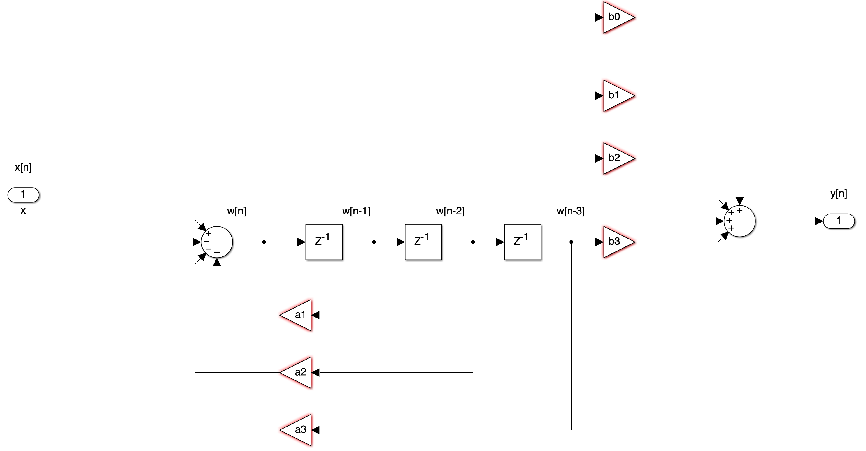
Fig. 14 Recursive digital filter realization in Simulink

Download Simulink model recursive.slx

Non-recursive realization

Fig. 15 shows a Simulink model of a third-order non-recursive realization of a digital filter2

nonrecursive

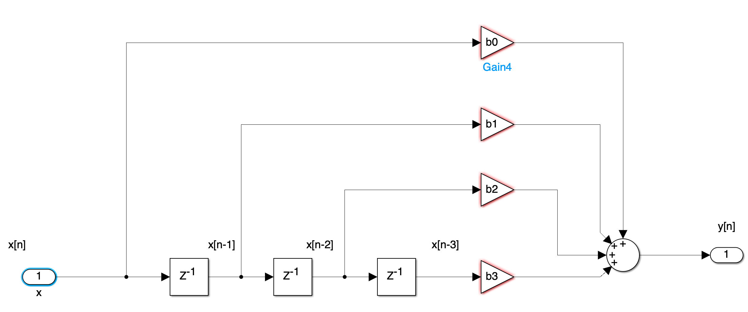
Fig. 15 Non-recursive digital filter realization in Simulink

Download Simulink model nonrecursive.slx

Generally, IIR filters are implemented by a recursive realization, and FIR filters are implemented by a non-recursive implementation.

Digital filter design methods

As demonstrated in Unit 7.1: Designing Analogue Filters, filter-design methods have been established and analogue prototypes have been published. Thus, we can choose an appropriate analogue prototype to satisfy the requirements.

Transformation methods are also available to transform analogue prototypes into an equivalent digital filter.

Three commonly used transformation methods are

1. The impulse invariant method

Produces a digital filter \(H(z)\) whose impulse response consists of the sampled values of the impulse response of the equivalent analogue filter \(H(s)\).

This is implemented in MATLAB by the system transformation function: Hz = c2d(Hs,Ts,'impulse') where Hs is the analogue transfer function \(H(s)\), Ts is the sampling period, and Hz is the equivalent \(H(z)\).

2. The step invariant method

Produces a digital filter \(H(z)\) whose step response consists of the sampled values of the step response of the equivalent analogue filter \(H(s)\).

3. The bilinear transformation method

This uses the transformation3

(39)\[s = \frac{2}{T_s}\cdot\frac{z-1}{z+1}\]

to transform the left-half of the \(s\)-plane into the interior of the unit circle in the \(z\)-plane.

In this unit, we will discuss, and assess, only the use of the blinear transformation.

The Bilinear Transformation

We recall from Relationship Between the Laplace and Z-Transform that since \(z = e^{sT_s}\), \(s = 1/T_s \log_e z\), then a DT transfer function \(H(z)\) can be determined from a CT transfer function \(H(s)\) using the mapping:

(40)\[H(z) = \left.H(s)\right|_{s = \frac{1}{T_s} \log_e z}\]

But the relation \(s = 1/T_s \log_e z\) is a multi-valued transformation, and as such, cannot be used to derive a rational polynomial in \(z\).

It can be approximated as

\[s = \frac{1}{T_s} \log_e z = \frac{2}{T_s} \left[\frac{z-1}{z+1} + \frac{1}{3} \left(\frac{z-1}{z+1} \right)^3 + \frac{1}{5} \left(\frac{z-1}{z+1} \right)^5 + \frac{1}{7} \left(\frac{z-1}{z+1} \right)^7 + \cdots\right]\]

(41)\[s \approx \frac{2}{T_s} \cdot \frac{z-1}{z+1} \]

Substitution of (41) into (40) yields

(42)\[H(z) = \left.G(s)\right|_{s = \frac{2}{T_s} \cdot \frac{z-1}{z+1}} \]

Digital frequency response of the bilinear transformation

The digital frequency response (using \(\omega_d\) on the unit circle in the \(z\)-plane) is obtained by the substitution \(z = e^{j\omega_d T_s}\), giving

(43)\[H\left(e^{j\omega_d T_s}\right) = H\left(\frac{2}{T_s} \cdot \frac{e^{j\omega_d T_s } - 1}{e^{j\omega_d T_s } + 1} \right) \]

Since the \(z\to s\) transformation maps the unit circle on the \(z\)-plane into the \(j\omega\) axis on the \(s\)-plane, the quantity

\[\frac{2}{T_s} \cdot \frac{e^{j\omega_d T_s } - 1}{e^{j\omega_d T_s} + 1}\]

and \(j\omega\) must be equal to some point \(\omega = \omega_a\) on the \(j\omega\) axis.

That is,

\[j\omega_a = \frac{2}{T_s} \cdot \frac{e^{j\omega_d T_s } - 1}{e^{j\omega_d T_s } + 1}\]

or

\[\omega_a = \frac{1}{J} \cdot \frac{2}{T_s} \cdot \frac{e^{j\omega_d T_s } - 1}{e^{j\omega_d T_s } + 1} = \frac{2}{T_s}\cdot \frac{1/(j2)}{1/2} \cdot \frac{e^{j\omega_d T_s/2} - e^{-j\omega_d T_s/2}}{e^{j\omega_d T_s/2} + e^{-j\omega_d T_s/2}}\]

\[\omega_a = \frac{2}{T_s} \cdot \frac{\sin\left(\omega_d T_s\right)/2}{\cos\left(\omega_d T_s\right)/2} \]

or

(44)\[\omega_a = \frac{2}{T_s} \tan\left(\frac{\omega_d T_s}{2} \right)\]

Frequency warping of the bilinear transformation

We see that the analogue frequency to digital frequency transformation results in a non-linear mapping; this condition is know as warping.

For instance, the frequency range \(0 \lt \omega_a \le \infty\) the analogue frequency is warped into the range \(0 \le \omega_d \le \pi/T_s\) in digital frequency.

To express \(\omega_d\) in terms of \(\omega_a\), we rewrite (44) as

\[\tan\left(\frac{\omega_d T_s}{2} \right) = \frac{\omega_a T_s}{2} \]

Then,

\[\omega_d T_s = 2 \tan^{-1}\left(\frac{\omega_a T_s}{2}\right) \]

and for small \(\omega_a T_s/2\),

\[\tan^{-1}\left(\frac{\omega_a T_s}{2}\right) \approx \frac{\omega_a T_s}{2}\]

Therefore,

(45)\[\omega_d T_s \approx 2 \left(\frac{\omega_a T_s}{2}\right) \approx \omega_a T_s\]

that is, for small frequencies,

(46)\[\omega_d \approx \omega_a\]

In MATLAB, \(z\) is a function of normalized frequency and thus the range of frequencies in \(H(z)\) is from \(0 \to \pi\). Then (45), when used with MATLAB, becomes

(47)\[\omega_d \approx \frac{\omega_a T_s}{\pi} \]

Pre-warping

The effect of warping can be eliminated by pre-warping the analogue filter prior to the application of the bilinear transformation. This is acomplished with the use of (44).

Example 12

Compute the transfer function \(H(z)\) of a low-pass filter with \(3\) dB cutoff frequency at \(20\) Hz, and attenuation of at least \(10\) dB for frequencies greater than \(40\) Hz. The sampling frequency \(f_s = 200\) Hz. Compare the magnitude plot with that obtained by a low-pass analogue filter with the same specifications.

Solution

We will apply the bilinear transformation. We arbitrarily choose a second-order Butterworth filter which will meet the stop-band specification.

The transfer function \(H(s)\) of the analogue low-pass filter with normalized frequency at \(\omega_c = 1\) rad/s is found with the MATLAB buttap function as follows:

 [z,p,k] = buttap(2); [b,a] = zp2tf(z,p,k)

b =
     0     0     1

a =
    1.0000    1.4142    1.0000

Thus, the transfer function with noramlized frequency, denoted as \(H_n(s)\), is

(49)\[H_n(s) = \frac{1}{s^2 + 1.414 s + 1} \]

Now, we must transform this transfer function to another with actual cutoff frequency at \(20\) Hz. We donote it as \(H_a(s)\).

We will first pre-warp the analogue frequency which by relation (44), us related to the digital frequency as

\[\omega_a = \frac{2}{T_s}\tan\left(\frac{\omega_d T_s}{2} \right)\]

where

\[T_s = \frac{1}{f_s} = \frac{1}{200}.\]

Denoting the analogue cutoff (3 dB) frequency as \(\omega_{ac}\), we obtain

\[\omega_{ac} = 400 \tan \left(\frac{2\pi\times 20}{2\times 200} \right) = 400\tan\left(0.1\pi\right) \approx 130\,\mathrm{rad/s}\]

or

\[f_{ac} = \frac{130}{2\pi} \approx 20.69\,\mathrm{Hz}.\]

As expected from relation (46), this frequency is very close to the discrete-time frequency \(f_{dc} = 20\) Hz, and thus from (49),

(49)\[H_a(s) \approx H_n(s) = \frac{1}{s^2 + 1.414 s + 1} \]

Relation (49) applies only when the cutoff frequency is normalized to \(\omega_c = 1\) rad/s.

If \(\omega_c \ne 1\), we must scale the transfer function in accordance with relation (33), that is,

\[H(s)_\mathrm{actual} = H\left(\frac{s}{\omega_\mathrm{actual}} \right) \]

For this example, \(\omega_\mathrm{actual} = 130\) rad/s, and thus we replace \(s\) with \(s/130\) and we obtain

\[H_a(s) = \frac{1}{\left(s/130\right)^2 + 1.414s/130 + 1} \]

We will use MATLAB to simplify this expression

syms s; simplifyFraction(1/((s/130)^2 + 1.414*s/130 + 1))
845000/50
9191/50

ans =

845000/(50*s^2 + 9191*s + 845000)

ans =
       16900

ans =
  183.8200

Then,

(50)\[H_a(s) = \frac{845000}{50s^2 + 9191s + 845000} = \frac{16900}{s^2 + 183.82s + 16900} \]

and making the substitution of \(s = (2/T_s)(z -1)/(z + 1) = 400(z-1)/(z + 1)\) we obtain

\[H(z) = \frac{16900}{\left(400\cdot \frac{z-1}{z + 1}\right)^2 + \frac{183.82\times 400(z-1)}{(z + 1)} + 16900} \]

We use the MATLAB code below to simplify this expression

syms z; simplify(16900/((400*(z-1)/(z+1))^2 + 183.82*400*(z - 1)/(z + 1) + 16900))

ans =

(4225*(z + 1)^2)/(62607*z^2 - 71550*z + 25843)

expand(4225*(z + 1)^2)

ans =

4225*z^2 + 8450*z + 4225

and thus

(51)\[H(z) = \frac{4225z^2 + 8450z + 4225}{62607z^2 - 71550z + 25843} \]

We will used the MATLAB freqz function to plot the magnitude of \(H(z)\), but we must first express it in negative powers of \(z\).

Dividing each term of (51) by \(62607z^2\), we obtain

(52)\[\frac{0.0675 + 0.1350z^{-1} + 0.0675z^{-2}}{1 - 1.1428z^{-1} + 0.4128 z^{-2}}\]

The MATLAB script below will generate \(H(z)\) and will plot the magnitude of this transfer function.

az = [1,  -1.1428, 0.4128]; bz = [0.0675, 0.1350, 0.0675]; fs = 200; fc = 20;
[Hz, wT] = freqz(bz,az,fc,fs);
semilogx(wT,20*log10(abs(Hz))); xlabel('Frequency in Hz - log scale')
ylabel('Magnitude (dB)'), title('Digital Low-Pass Filter. Example 12'),grid

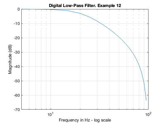
We now plot the analogue equivalent to compare the digital to the analogue frequency response.

The MATLAB script below produces the desired plot.

[z,p,k] = buttap(2); [b, a] = zp2tf(z,p,k); f = 1:1:100; fc = 20; [bn,an] = lp2lp(b,a,fc);
Hs = freqs(bn,an,f);
semilogx(f, 20*log10(abs(Hs))), xlabel('Frequency in Hz - log scale')
ylabel('Magnitude (dB)'), title('Analogue Low-Pass Filter. Example 12'),grid

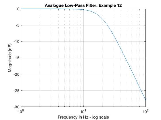
Comparing the digital filter plot with the equivalent analogue filter plot, we observe that the magnitude is greater than \(-3\) dB for frequencies less than \(20\) rad/s, and is smaller than \(-10\) dB for frequencies greater than \(40\) Hz. Therefore, both the digital and analogue low-pass filters meet the specified requirements.4

MATLAB bilinear function

An analogue filter transfer function can be mapped to a digital transfer function directly with the MATLAB bilinear function. The procedure is illustrated with the following example.

Example 13

Use the MATLAB bilinear function to derive the low-pass digital transfer function \(H(z)\) from a second-order Butterworth analogue filter with a \(3\) dB cutoff frequency at \(50\) Hz, and sample rate \(f_s = 500\) Hz.

Solution

We will use the following MATLAB script to produce the desired digital filter function:

[z,p,k] = buttap(2); [num,den] = zp2tf(z,p,k); fc = 50; wc = 2*pi*fc;
[num1,den1] = lp2lp(num,den,wc);
fs = 500; [numd,dend] = bilinear(num1, den1, fs)

numd =
    0.0640    0.1279    0.0640

dend =
    1.0000   -1.1683    0.4241

Therefore, the transfer function \(H(z)\) for this filter is

(53)\[H(z) = \frac{0.0640 z^2 + 0.1279 z + 0.0640}{z^2 -1.1683 z + 0.4241} = \frac{0.0640 + 0.1279 z^{-1} + 0.0640 z^{-2}}{1 -1.1683 z^{-1} + 0.4241 z^{-2}}\]

MATLAB Functions for direct digital filter design

MATLAB provides us with a suite of functions that we need to design digital filters using analogue prototypes. These are listed below.

• N = order of the filter

• Wn = normalized cutoff frequency

• Rp = pass band ripple

• Rs = stop band ripple

• B = \(B(z)\), i.e. the numerator of the discrete transfer function \(H(z) = B(z)/A(z)\)

• A = \(A(z)\), i.e. the denominator of the discrete transfer function \(H(z)\)

The MathWorks also provides a catalogue of filter design tools with examples in the Filter Design Gallery.

For Low-Pass Filters

[B,A] = butter(N,Wn)
[B,A] = cheb1(N,Rp,Wn)
[B,A] = cheb2(N,Rs,Wn)
[B,A] = ellip(N,Rp,Rs,Wn)

For High-Pass Filters

[B,A] = butter(N,Wn,'high')
[B,A] = cheb1(N,Rp,Wn,'high')
[B,A] = cheb2(N,Rs,Wn,'high')
[B,A] = ellip(N,rp,Rs,Wn,'high')

For Band-Pass Filters

[B,A] = butter(N,[Wn1,Wn2])
[B,A] = cheb1(N,Rp,[Wn1,Wn2])
[B,A] = cheb2(N,Rs,[Wn1,Wn2])
[B,A] = ellip(N,Rp,Rs,[Wn1,Wn2])

For Band-Elimination Filters

[B,A] = butter(N,[Wn1,Wn2],'stop')
[B,A] = cheb1(N,Rp,[Wn1,Wn2],'stop')
[B,A] = cheb2(N,Rs,[Wn1,Wn2],'stop')
[B,A] = ellip(N,Rp,Rs,[Wn1,Wn2],'stop')

Example 13

The transfer functions (53) through (56), describe different types of digital filters. Use the MATLAB freqz commmand to plot the magnitude versus radian frequency. What types of filter does each transfer function represent? What classes of filter are they?

13(a)

(54)\[H_1(z) = \frac{\left(2.8982 + 8.6946z^{-1} + 8.6946z^{-2} + 2.8982z^{-3}\right)\cdot 10^{-3}}{1 - 2.3741z^{-1} + 1.9294z^{-2} - 0.5321z^{-3}} \]

13(b)

(55)\[H_2(z) = \frac{0.5276 - 1.5828z^{-1} + 1.5828z^{-2} - 0.5276z^{-3}}{1 - 1.7600z^{-1} + 1.1829z^{-2} - 0.2781z^{-3}} \]

13(c)

(56)\[H_3(z) = \frac{\left(6.8482 - 13.6964z^{-2} + 6.8482z^{-4}\right)\cdot 10^{-4}}{1 + 3.3033z^{-1} + 4.5244z^{-2} + 3.1390z^{-3} + 0.9603z^{-4}}\]

13(d)

(57)\[H_4(z) = \frac{0.9270-1.2079z^{-1}+0.9270z^{-2}}{1-1.2079z^{-1}+0.8541z^{-2}} \]

Solution

The MATLAB script to plot each of the transfer functions of (53) through (56), is given below where N = 512, i.e. the default value.

b1 = [2.8982, 8.6946, 8.6946, 2.8982]*10^(-3); a1 = [1, -2.3741, 1.9294, -0.5321];
[H1z,w1T] = freqz(b1, a1);

b2 = [0.5276, -1.5828, 1.5828, -0.5276]; a2 = [1, -1.7600, 1.1829, -0.2781];
[H2z,w2T] = freqz(b2, a2);

b3 = [6.8482, 0, -13.6964, 0, 6.8482]*10^(-4); a3 = [1, 3.2033, 4.5244, 3.1390, 0.9603];
[H3z,w3T] = freqz(b3, a3);

b4 = [0.9270, -1.2079, 0.9270]; a4 = [1, -1.2079, 0.8541];
[H4z,w4T] = freqz(b4, a4);

Now do the plots

clf; % clear the current figure
subplot(221), semilogx(w1T,abs(H1z)),axis([0.1 1 0 1]),title('Filter for H1(z)')
xlabel(''),ylabel('Magnitude'),grid
%
subplot(222), semilogx(w2T,abs(H2z)),axis([0.1 10 0 1]),title('Filter for H2(z)')
xlabel(''),ylabel('Magnitude'),grid
%
subplot(223), semilogx(w3T,abs(H3z)),axis([1 10 0 1]),title('Filter for H3(z)')
xlabel(''),ylabel('Magnitude'),grid
%
subplot(224), semilogx(w4T,abs(H4z)),axis([0.1 10 0 1]),title('Filter for H4(z)')
xlabel(''),ylabel('Magnitude'),grid

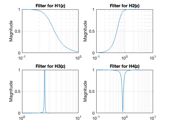
It is clear that the filters are low-pass, high-pass, band-pass and band-stop. There is now ripple in the pass-band or stop band so they are all Butterworth filters.

Digital Filter Design with Simulink

As stated earlier in this unit, a digital filter is a computational process, or algorithm, that converts one sequence of numbers representing the input signal into another sequence of numbers representing the output signal.

To close out this unit and the module, we will explore Simulink models that can be used to implement digital filters, and present the Digital Filter Design block included in the Simulink DSP System Toolbox, which can generate these models automatically.

The Direct Form I Realization of a Digital Filter

The Direct Form I Realization of a second-order digital filter is shown in Fig. 16.

dfir_df

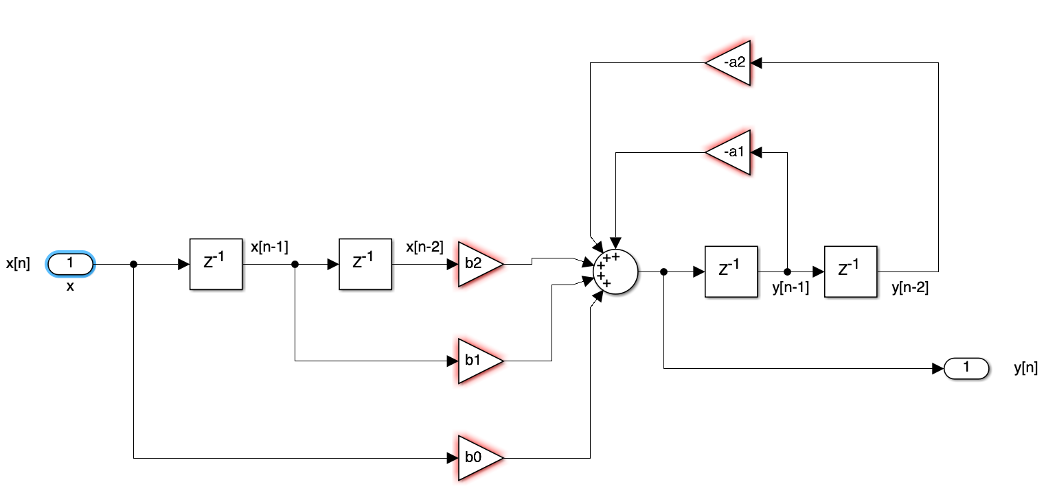
Fig. 16 Direct Form I Realization of a second-order digital filter

Download this model as dfir_df.

At the summing junction of Fig. 16 we obtain

\[b_0X(z)+b_1z^{-1}X(z)+b_2z^{-2}X(z) + \left(-a_1\right)z^{-1}Y(z) + \left(-a_1\right)z^{-2}Y(z) = Y(z)\]

\[X(z)\left(b_0 + b_1z^{-1} + b_2z^{-2}\right) = Y(s)\left(1 + a_1z^{-1} + a_2z^{-2}\right)\]

And thus, the transfer function of the Direct Form I Realization of the second-order digital filter of Fig. 16 is

(58)\[H(z) = \frac{Y(z)}{X(z)} = \frac{b_0 + b_1z^{-1} + b_2z^{-2}}{1 + a_1z^{-1} + a_2z^{-2}} \]

A disadvantage of the Direct Form I Realization digital filter is that it requires \(2k\) registers where \(k\) represents the order of the filter. We observe that the second-order (\(k=2\)) digital filter of Fig. 16 requires 4 delay (register) elements denoted as \(z^{-1}\). However, this form of realization has the advantage that there is no possibility of internal filter overflow5.

The Direct Form II Realization of a Digital Filter

The Direct Form II Realization6 of a second-order digital filter is shown in Fig. 17. The Simulink Transfer Fcn Direct Form II block implements the transfer function of this filter.

dfiir_df

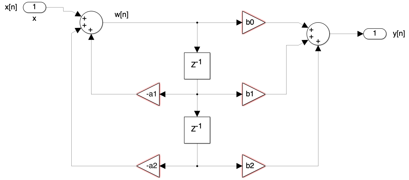
Fig. 17 Direct Form II Realization of a second-order digital filter

Download this model as dfiir_df.slx.

The transfer function for the Direct Form-II second-order digital filter of Fig. 17 is the same as for a Direct Form-I second-order filter of Fig. 16, that is,

(59)\[H(z) = \frac{b_0 + b_1z^{-1} + b_2z^{-2}}{1 + a_1z^{-1} + a_2z^{-2}} \]

A comparison of (58) and (59) shows that whereas a Direct Form-I second-order digital filter requires \(2k\) registers, where \(k\) represents the order of the filter, a Direct Type-II second-order digital filter requires only \(k\) register elements denoted as \(z^{-1}\). This is because the register (\(z^{-1}\)) elements of the Direct Form-II realization are shared between the zeros section and the poles section.

Example 14

Fig. 18 shows a Direct Form-II second-order digital filter whose transfer function is

(60)\[H(z) = \frac{1+1.5z^{-1}+1.02z^{-2}}{1 - 0.25 z^{-1} -0.75 z^{-2}} \]

ex14

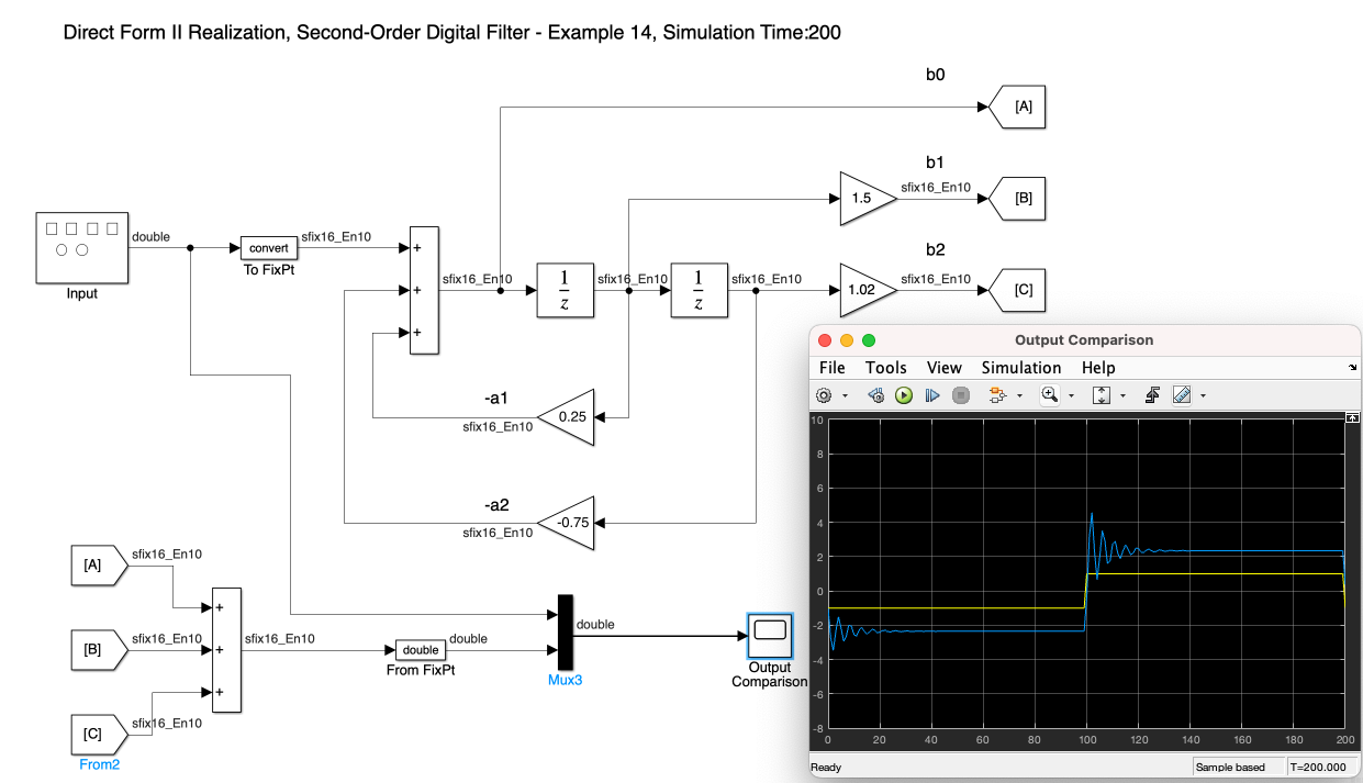
Fig. 18 Model for Example 14

Download this model as ex14.slx.

The Series Form Realization of a Digital Filter

For the Series Form Realization, the transfer function is expressed as a product of first-order and second-orer transefer functions as shown in (61) below.

(61)\[H(z) = H_1(z)\cdot H_2(z)\cdots H_R(z)\]

Relation (61) is implemented as the cascaded blocks shown in Fig. 19.

Fig. 19 Series Form Realization

Fig. 20 shows the Series Form Realization of a second-order digital filter.

series_form_2nd

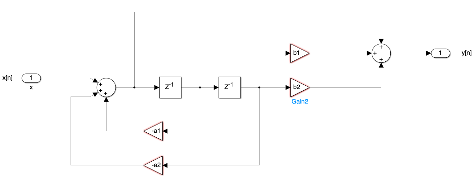
Fig. 20 Series Form Realization of a second-order digital filter

Download this model as series_form_2nd.slx.

Example 15

The transfer function of the series form Realization of a certian second-order digital filter is

\[H(z) = \frac{0.5\left(1-0.36z^{-2}\right)}{1 + 0.1 z^{-1} - 0.72 z^{-2}} \]

To implement this filter, we factor the numerator and denominator polynomials as7

(62)\[H(z) = \frac{0.5\left(1+0.6z^{-1}\right)\left(1-0.6z^{-1}\right)}{\left(1+0.9z^{-1}\right)\left(1-0.8z^{-1}\right)} \]

The Simulink model and the input and output waveforms are shown in Fig. 21.

ex15

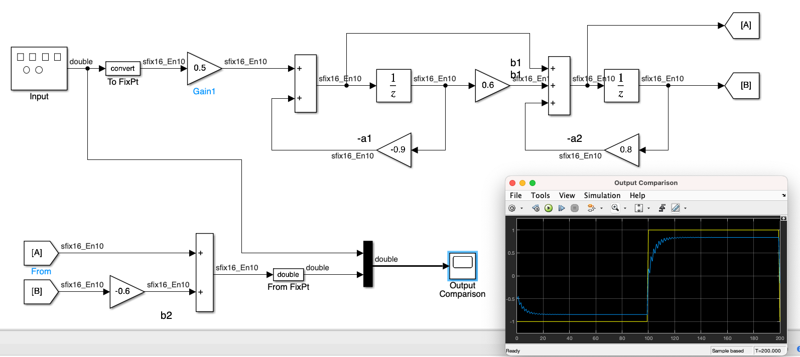
Fig. 21 Model for Example 15

Download this model as ex15.slx.

The Parallel Form Realization of a Digital Filter

The general form of the transfer function of a Parallel Form Realization is

(63)\[H(z) = K + H_1(z) + H_2(z) + \cdots + H_R(z)\]

Relation (63) is implemented as the parallel blocks shown in Fig. 22.

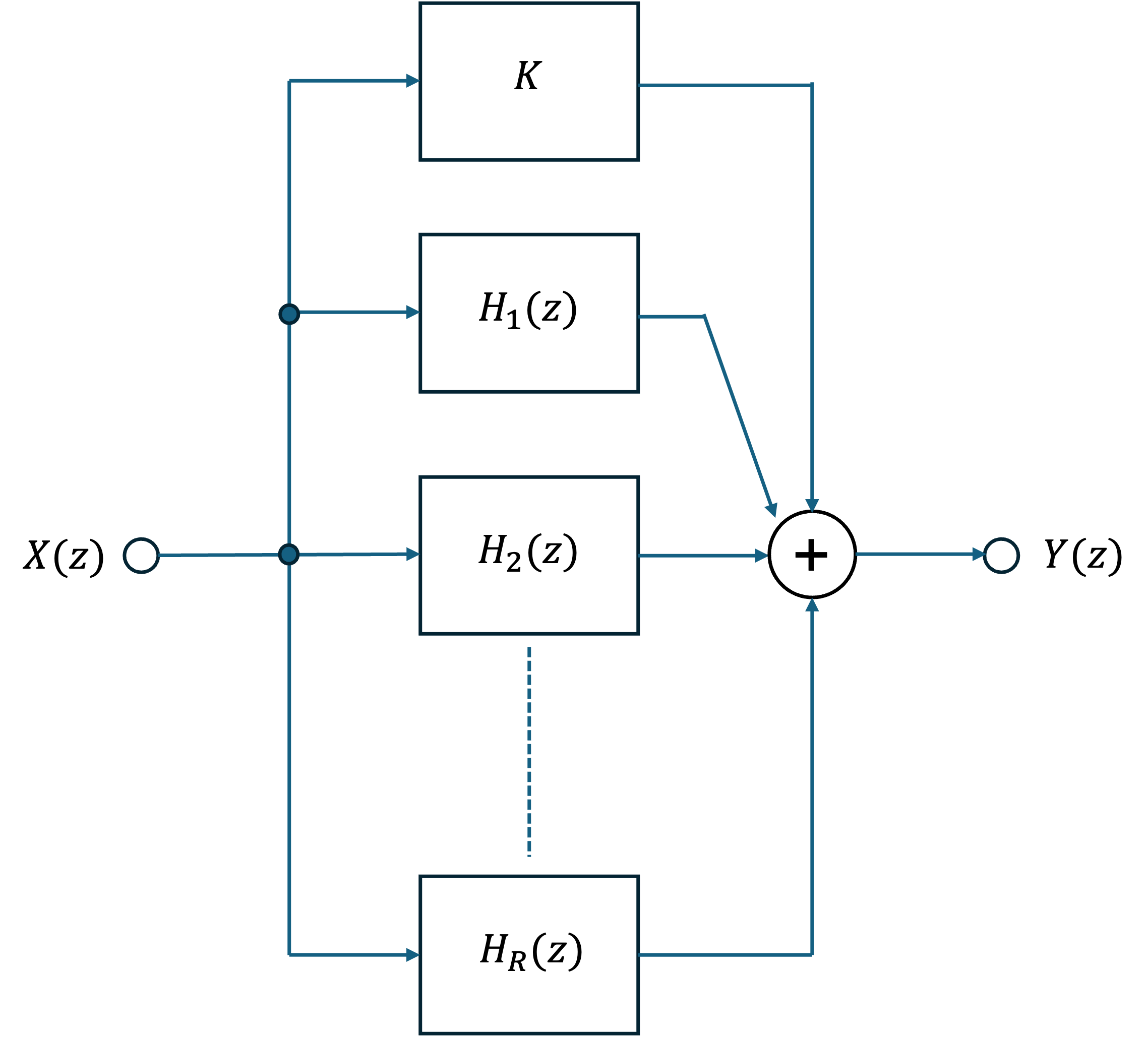
Fig. 22 Parallel Form Realization of a second-order digital filter

As with the Series Form Realization, the ordering of the individual filters in Fig. 22 is immaterial. But because of the presence of the constant \(K\), we can simplify the transfer function expression by performing the partial fraction expansion after we express the transfer function in the form \(H(z)/z\).

Example 16

The transfer function of a certain second-order digital filter is

\[H(z) = \frac{0.5\left(1-0.36z^{-2}\right)}{1+0.1z^{-1}-0.72z^{-2}} \]

Implement this filter using the Parallel Form Realization.

\[\frac{H(z)}{z} = \frac{0.5\left(z+0.6\right)\left(z-0.6\right)}{z\left(z+0.9\right)\left(z-0.8\right)} \]

Next we perform partial fraction expansion

\[\frac{0.5\left(z+0.6\right)\left(z-0.6\right)}{z\left(z+0.9\right)\left(z-0.8\right)} = \frac{r_1}{z} + \frac{r_2}{z+0.9} + \frac{r_2}{z-0.8} \]

\[r_1 = \left.\frac{0.5\left(z+0.6\right)\left(z-0.6\right)}{\left(z+0.9\right)\left(z-0.8\right)}\right|_{z=0} = 0.25\]

\[r_2 = \left.\frac{0.5\left(z+0.6\right)\left(z-0.6\right)}{z\left(z-0.8\right)}\right|_{z=-0.9} = 0.147\]

\[r_3 = \left.\frac{0.5\left(z+0.6\right)\left(z-0.6\right)}{z\left(z+0.9\right)}\right|_{z=0.8} = 0.103\]

Therefore,

\[\frac{H(z)}{z} = \frac{0.25}{z} + \frac{0.147}{z+0.9} + \frac{0.103}{z-0.8}\]

\[H(z) = 0.25 + \frac{0.147z}{z+0.9} + \frac{0.103z}{z-0.8}\]

(64)\[H(z) = 0.25 + \frac{0.147}{1+0.9z^{-1}} + \frac{0.103}{1-0.8z^{-1}}\]

The model and input and output waveforms are shown in Fig. 23.

ex16

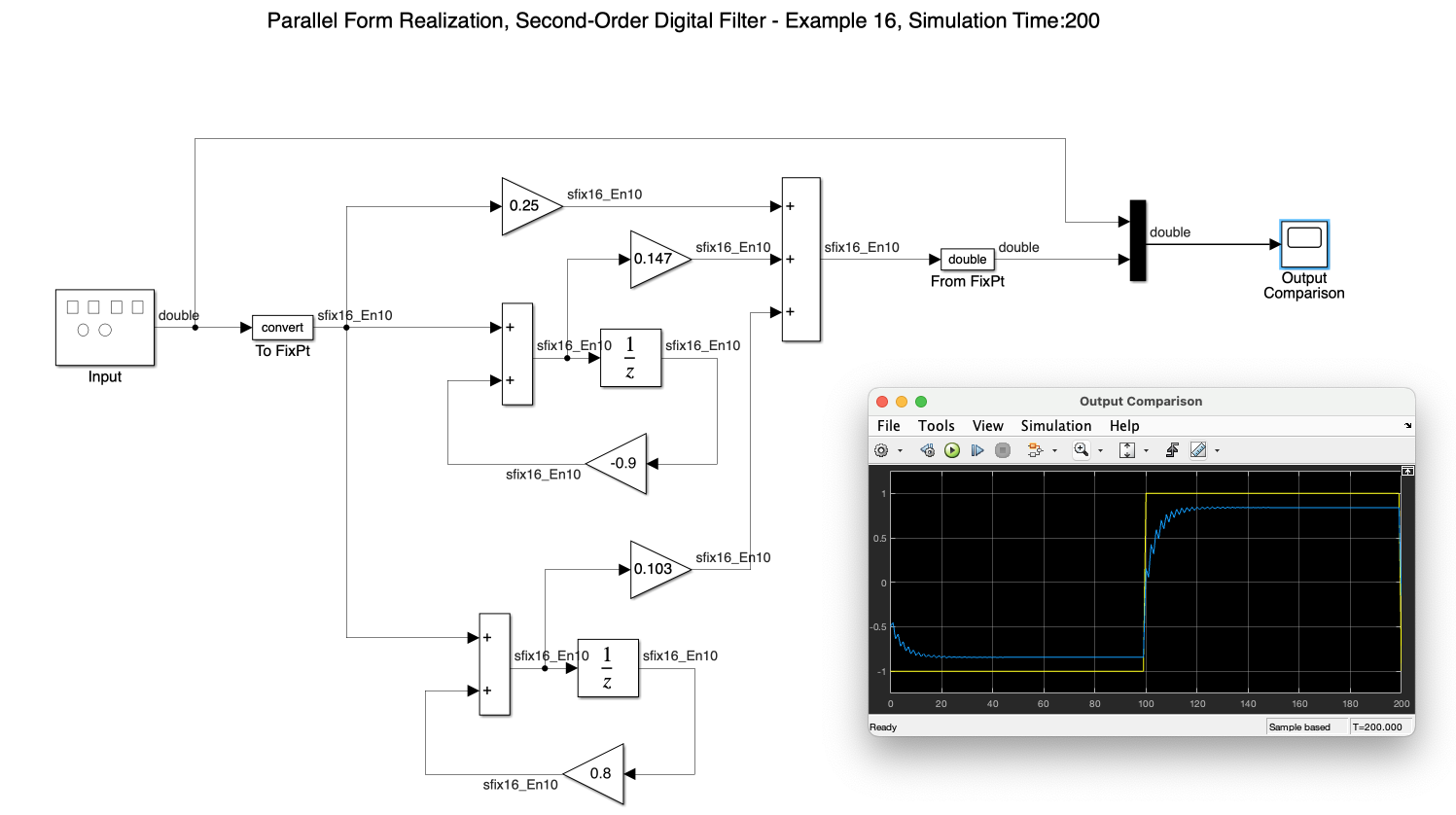
Fig. 23 Model for Example 16

Download this model as ex16.slx.

The Digital Filter Design Block

The Digital Filter Design block is included in the DSP System Toolbox and is included in the version of MATLAB for which Swansea University has a site license. It also works on MATLAB online. This block can be used to create models related to digital filter design applications directly in Simulink.

The functionality of this block can be observed by dragging this block from the library into a model and double clicking it.

dfd_block

When this is done, the Block Parameters dialogue box appears as shown in Fig. 24.

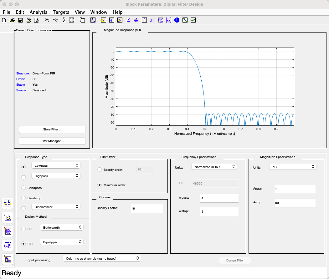
Fig. 24 The Digital Filter Design Block Parameters dialogue box

Download this model as ex16.slx.

As indicated on the lower left part of this window, we can choose the Response Type (Low-Pass, High-Pass, Band-Pass or Band-Stop), the Design Method (IIR or FIR) where an IIR filter can be Butterworth, Chebyshev Type I, Chebyshev Type II, or Elliptic, and FIR can be Window, Maximally Flat, etc., and the Window8 can be Kaiser, Hamming etc. We must click on the Design Filter. buttom at the bottom right of the Block Parameters dialogue box to update the specifications.

We will not give an actual example of the use of the Simulink filter design block in these notes. Instead we refer you to Example 11.7 in [Karris, 2012] and also to the relevant page Using Digital Filter Design Block in the MATLAB documentation site. There you will find documentation of the Digital Filter Design Block and several examples of its use.

If you go on from this course to do some actual signal processing, we would urge you to take full advantage of these resources.

Code generation

As well as the ability to design filters that can be immediately used in simulations of digital signal processing applications, and the muliple analysis tools it provides in the the Digital Filter Design Block, povided by the Signal Processing Toolbox and the DSP System Toolbox, be used for code generation.

For example, it can generate Simulink models of the designed filter, as well as C header files, and HDL code for VHDL and verilog devices.

Thus, MATLAB can be used in a so-called model-based design process as described in the opening video

The End?

This concludes this module. Don’t forget to let us know how it went for you in the end of module feedback.

There are exercises in the notes which will give you practice in the sort of questions that will come up in the exam.

Hopefully you found the module interesting and will make use of some of your knowledge after the exams are over!

Exercises

Exercise 7.2.1

Exam Preparation

Use the block diagram shown in Fig. 14 to validate (38) and (37).

Solution to Exercise 7.2.1

Exam Preparation

Exercise 7.2.2

Use the block diagram shown in Fig. 17 to validate (55). Write down the equivalent difference equation.

Solution to Exercise 7.2.2

Exercise 7.2.3

Exam Preparation

Design a 2nd-order Butterworth filter with \(\omega_c = 20\) kHz. Use the Bilinear transformation to convert the analogue filter to a digital filter with sampling frequency of 44.1 kHz. Use pre-warping to ensure that the cutoff frequency is correct at the equivalent digital frequency.

Solution to Exercise 7.2.3

Exercise 7.2.4

Exam Preparation

A digital filter with cutoff frequency of 100 Hz for a signal sampled at 1 kHz has transfer function

\[H(z) = \frac{0.6401 -1.1518z^{-1} + 0.6401z^{-2}}{1 -1.0130 z^{-1} + 0.4190z^{-2}} \]

The frequency response for this filter (plotted against \(f/(f_s/2)\)) is shown in Fig. 25.

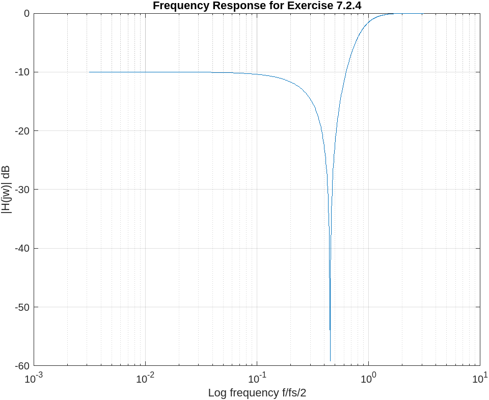
Fig. 25 Frequency response for Example 7.2.4

a) What type of filter is this?

b) Estimate the band-pass ripple, and stop-band ripple of the filter.

c) Implement the filter as Direct Form Type II digital filter and sketch its block diagram.

d) Use the example of Convert to code to give a code implementation of the filter.

e) If the input to this filter is a step function \(x[n] = \left\{1,1,1,1,\ldots\right\}\), calculate the first 5 outputs \(y[n]\) of the filter.

Solution to Exercise 7.2.4

References

See Bibliography.

Footnotes

---

1

Note that the block labelled \(z^{-1}\) is a one unit delay \(y[n] = x[n - 1]\); the triangular blocks are gains \(y[n] = k x[n]\); and the circular blocks are summing points. Following the equations we have \(w[n] = x[n] - a_1 w[n-1] - a_2 w[n-2] - a_3 w[n-3]\) and \(y[n] = b_0 w[n] + b_1 w[n-1] + b_2 w[n-2] + b_3 w[n-3]\). It is left as an exercise for the reader to show that combining these two equations, taking Z-transforms, and eliminating \(W(z)\), results in the transfer function \(H(z) = Y(z)/X(z)\) given in (38) and hence the difference equation of (37).

2

It is obvious from this figure that \(y[n] = b_0 x[n] + b_1 x[n-1] + b_2 x[n-2] + b_3 x[n-3]\).

3

\(T_s\) is the sampling period, that is the reciprocal of the sampling frequency \(f_s\) Hz.

4

Note the significant distortion of the digital filter response at high frequencies.

5

For a detailed discussion on overflow conditions please refer to Section 10.5, Chapter 10, Page 10-6 of [Karris, 2005].

6

The Direct Form-II is also known as the Canonical Form.

7

The way we combine the numerator and denominator factors is immaterial. For example we could group the factors as \(\left(1 + 0.6z^{-1}\right)/\left(1+0.9z^{-1}\right)\) and \(\left(1 - 0.6z^{-1}\right)/\left(1-0.8z^{-1}\right)\), or as \(\left(1 + 0.6z^{-1}\right)/\left(1-0.8z^{-1}\right)\) and \(\left(1 - 0.6z^{-1}\right)/\left(1+0.9z^{-1}\right)\).

8

A window function multiplies the infinte length impulse response (IIR) by a finite width function, referred to a a window function, so that the infinite length series will be terminated after a finite number of terms in the series. This causes what is called leakage and results in additional ripple in the frequency domain. Windows of various shapes can be used to minimize this leakage for particular applications. The study of windowing functions is beyond the scope of this course. In the CPD course Signal Processing Toolbox you were shown the use of windowing functions as a design method for approximating an ideal filter. EEE stidents will have experienced windowing effecrs in the EGA223 lab on ADC, DAC and filters. You can study windowing in more detail in Appendix E of [Karris, 2012].