Worked Solutions to Exercises 7.2

Worked Solutions to Exercises 7.2#

Solution to Exercise 7.2.1#

We first write down the difference equations by tracing through the signals in the block diagram of Fig. 15.

(66)#

y [n] = b_{0} w [n] + b_{1} w [n - 1] + b_{2} w [n - 2] + b_{3} w [n - 2]

(67)#

w [n] = x [n] - a_{1} w [n - 1] - a_{1} w [n - 2] - a_{3} w [n - 2]

We take Z-transforms of equations (66) and (67):

(68)#

Y (z) = b_{0} W (z) + b_{1} z^{- 1} W (z) + b_{2} z^{- 2} W (z) + b_{3} z^{- 3} W (z)

(69)#

W (z) = X (z) + a_{1} z^{- 1} W (z) + a_{1} z^{- 2} W (z) + a_{3} z^{- 3} W (z)

Gather terms in (68) and (69):

(70)#

Y (z) = (b_{0} + b_{1} z^{- 1} + b_{2} z^{- 2} + b_{3} z^{- 3}) W (z)

(71)#

(1 + a_{1} z^{- 1} - a_{1} z^{- 2} - a_{3} z^{- 3}) W (z) = X (z)

From (71) we obtain

(72)#

W (z) = \frac{1}{1 + a_{1} z^{- 1} - a_{1} z^{- 2} - a_{3} z^{- 3}} X (z)

We then use (72) to eliminate $W (z)$ from (70), giving

Y (z) = \frac{b_{0} W (z) + b_{1} z^{- 1} W (z) + b_{2} z^{- 2} W (z) + b_{3} z^{- 3}}{1 + a_{1} z^{- 1} - a_{1} z^{- 2} - a_{3} z^{- 3}} X (z)

and the transfer function follows:

(73)#

H (z) = \frac{Y (z)}{X (z)} = \frac{b_{0} W (z) + b_{1} z^{- 1} W (z) + b_{2} z^{- 2} W (z) + b_{3} z^{- 3}}{1 + a_{1} z^{- 1} - a_{1} z^{- 2} - a_{3} z^{- 3}}

Solution to Exercise 7.2.2#

Use the block diagram shown in Fig. 18 to validate (54). Write down the equivalent difference equation.

See: u72:ex:2

The same procedure used for Solution to Exercise 7.2.1 is used.

Solution to Exercise 7.2.3#

Design a 2nd-order Butterworth filter with $ω_{c} = 20$ kHz. Use the Bilinear transformation to convert the analogue filter to a digital filter with sampling frequency of 44.1 kHz. Use pre-warping to ensure that the cutoff frequency is correct at the equivalent digital frequency.

See: Exercise 7.2.3

The magnitude squared function of a $k$ -th order Butterworth low-pass filter is

A^{2} (ω) = \frac{1}{(ω / ω_{c})^{2} k + 1)}

We need to design a filter that has $k = 2$ and $ω_{c} = 2 \times π \times 20 \times 10^{3} = 125, 66371 \times 10^{3}$ rad/s. It will be easier to design the filter for $ω_{c} = 1$ then complete the design by subsitution of the actual cut-off frequency afterwards.

We follow the procedure outlined in the notes (see Butterworth Analogue Low-Pass Filter Design).

A^{2} (ω) = \frac{1}{ω^{4} + 1}

which on subsitution of $ω^{2} = - s^{2}$ gives

G (s) G (- s) = \frac{1}{s^{4} + 1}

The poles of this equation are given by $s = \sqrt[4]{- 1}$ , that is $s = \sqrt[4]{1 ∠ 180^{\circ}}$ which, by De Moivre’s theorem, with $n = 4$ ,

\sqrt[4]{1 e^{j π}} = 1 e^{j (\frac{π + 2 k π}{4})}

Thus $ $\begin{array}{ll} s_{1} = e^{j 3 π / 4} = - \frac{1}{\sqrt{2}} + j \frac{1}{\sqrt{2}} & s_{2} = e^{j 5 π / 4} = - \frac{1}{\sqrt{2}} - j \frac{1}{\sqrt{2}} \\ s_{3} = e^{j 7 π / 4} = + \frac{1}{\sqrt{2}} - j \frac{1}{\sqrt{2}} & s_{4} = e^{j 9 π / 4} = + \frac{1}{\sqrt{2}} + j \frac{1}{\sqrt{2}} \end{array}$ $

We take the left-half plane poles $s_{1}$ and $s_{2}$ and

H (s) = \frac{K}{(s + \frac{1}{\sqrt{2}} + j \frac{1}{\sqrt{2}}) (s + \frac{1}{\sqrt{2}} + j \frac{1}{\sqrt{2}})}

H (s) = \frac{K}{s^{2} + \sqrt{2} s + 1}

The gain $K$ is found from $A^{2} (0) = 1$ , and $H (0) = 1$ , so $K = 1$ and the prototype Butterworth low-pass filter is

H (s) = \frac{1}{s^{2} + \sqrt{2} s + 1}

We now convert this to the filter we need by substitution $s = s / ω_{c}$

H (s) = \frac{1}{{(\frac{s}{ω_{c}})}^{2} + \sqrt{2} (\frac{s}{ω_{c}}) + 1}

from which

\frac{ω_{c}^{2}}{s^{2} + \sqrt{2} ω_{c} s + ω_{c}^{2}}

and

\frac{15.79 \times 10^{3}}{s^{2} + 177.7 s + 15.79 \times 10^{3}}

We will complete the problem by switching to MATLAB. We first need to determine the pre-warping correction

ω_{a} = \frac{2}{T_{s}} \tan (\frac{ω_{c} T_{s}}{2})

fs = 44.1e2; % sampling frequency
Ts = 1/fs;
wc = 2*pi*20e3

wc =

   1.2566e+05

wa = (2/Ts)*tan(wc*Ts/2)

wa =

  -7.9553e+04

Re calculate Butterworth filter with pre-warped frequency

Hs = tf(wa^2,[1 sqrt(2)*wa wa^2])

Hs =
 
           6.329e09
  ---------------------------
  s^2 - 1.125e05 s + 6.329e09
 
Continuous-time transfer function.

Now find $H (z)$ using the bilinear transformation by substituting

s = \frac{2}{T s} (\frac{z - 1}{z + 1})

You should try this algebraicly, but we will cheat

Hz = c2d(Hs,Ts,'tustin')

Hz =
 
  1.169 z^2 + 2.338 z + 1.169
  ---------------------------
     z^2 + 2.309 z + 1.367
 
Sample time: 0.00022676 seconds
Discrete-time transfer function.

From which

H (z) = \frac{1.169 z^{2} + 2.338 z + 1.169}{z^{2} + 2.309 z + 1.367}

To implement this, we simply convert to negative powers of $z$

H (z) = \frac{1.169 + 2.338 z^{- 1} + 1.169 z^{- 2}}{1 + 2.309 z^{- 1} + 1.367 z^{- 2}}

Solution to Exercise 7.2.4#

A digital filter with cutoff frequency of 100 Hz for a signal sampled at 1 kHz has transfer function

$H (z) = \frac{0.6401 - 1.1518 z^{- 1} + 0.6401 z^{- 2}}{1 - 1.0130 z^{- 1} + 0.4190 z^{- 2}}$

The frequency response for this filter (plotted against $f / (f_{s} / 2)$ ) is shown in Fig. 26.

a) What type of filter is this?

b) Estimate the band-pass ripple, and stop-band ripple of the filter.

c) Implement the filter as Direct Form Type II digital filter and sketch its block diagram.

d) Use the example of Convert to code to give a code implementation of the filter.

e) If the input to this filter is a step function $x [n] = {1, 1, 1, 1, \dots}$ , calculate the first 5 outputs $y [n]$ of the filter.

See: Exercise 7.2.4

This is a 2nd-order filter designed to have a cut-off frequency of $100$ Hz. Beacuse it is low-order, the ripple is rather non-typical!

a) The gain at high frequency is 0 dB so the filter is high-pass. There is ripple in the stop-band so it is Chebyshev Type II.

b) The stop-band ripple is 10 dB, there is no ripple in the pass-band. Note that it is not clear that the cut-off frequency is 100 Hz! Any value near the -3dB cut-off frequency will be taken as correct.

c) For the sketch, refer to Fig. 18 and note that the coefficients will be: $b_{0} = 0.6401$ , $b_{1} = - 1.1518$ , $b_{3} = 0.6401$ , $a_{1} = 1.0130$ , $a_{2} = 0.4190$ . Note in particular the signs of the $a$ coefficients. They are negative in the block diagram but positive in the transfer function.

d) To write the code, we need to express the transfer function as a difference equation.

H (z) = \frac{Y (z)}{X (z)} = \frac{0.6401 - 1.1518 z^{- 1} + 0.6401 z^{- 2}}{1 - 1.0130 z^{- 1} + 0.4190 z^{- 2}}

So

\begin{array}{r} \begin{aligned} (1 - 1.0130 z^{- 1} + 0.4190 z^{- 2}) Y (z) & = (0.6401 - 1.1518 z^{- 1} + 0.6401 z^{- 2}) X (z) \\ Y (z) - 1.0130 z^{- 1} Y (z) + 0.4190 z^{- 2} Y (z) & = 0.6401 X (z) - 1.1518 z^{- 1} X (z) + 0.6401 z^{- 2} X (z) \\ Y (z) & = 0.6401 X (z) - 1.1518 z^{- 1} X (z) + 0.6401 z^{- 2} X (z) + 1.0130 z^{- 1} Y (z) - 0.4190 z^{- 2} Y (z) \end{aligned} \end{array}

Taking inverse Z-transform:

y [n] = 0.6401 x [n] - 1.1518 x [n - 1] + 0.6401 x [n - 2] + 1.0130 y [n - 1] - 0.4190 y [n - 2]

Using the example in Convert to code with $T_{s} = 1 / 1000 = 0.001$

/* Initialize */
Ts = 0.001; /* more probably some fraction of clock speed */
ynm1 = 0; ynm2 = 0; unm1 = 0; unm2 = 0;
while (true) {
    un = read_adc();
    yn = 0.6401*un + −1.1518*unm1 + 0.6401*unm2 + 1.0130*ynm1 - 0.4190*ynm2;
    write_dac(yn);
    /* store past values */
    ynm2 = ynm1; ynm1 = yn;
    unm2 = unm1; unm1 = un;
    wait(Ts);
}

e) The easiest way to complete the problem is to tabulate the data

$n$	$x [n]$	$0.6401 x [n]$	$- 1.1518 x [n - 1]$	$0.6401 x [n - 2]$	$1.0130 y [n - 1]$	$- 0.4190 y [n - 2]$	$y [n]$
$0$	$1$	$0.6401$	$0$	$0$	$0$	$0$	$0.6401$
$1$	$1$	$0.6401$	$- 1.1518$	$0$	$0.6486$	$0$	$0.1369$
$2$	$1$	$0.6401$	$- 1.1518$	$0.6401$	$0.1387$	$- 0.2682$	$- 0.011$
$3$	$1$	$0.6401$	$- 1.1518$	$0.6401$	$- 0.0011$	$- 0.0574$	$0.0700$
$4$	$1$	$0.6401$	$- 1.1518$	$0.6401$	$0.0709$	$0.0004$	$0.1997$

from which $y [n] = {0.6401, 0.1369, - 0.011, 0.0700, 0.1997, \dots}$

I find the use of Excel to be a useful tool for confirming such results and the sheet for this one can be downloaded sol_ex_7_2_3.xlsx.

You can also use MATLAB of course. Here we set up the transfer function:

fs = 1000;
Ts = 1/fs
Hz = tf([0.6401,-1.1518,0.6401],[1,-1.0130,0.4190],Ts)

Ts =

   1.0000e-03


Hz =
 
  0.6401 z^2 - 1.152 z + 0.6401
  -----------------------------
      z^2 - 1.013 z + 0.419
 
Sample time: 0.001 seconds
Discrete-time transfer function.

Then compute the step response

[yn,nTs] = step(Hz);
stem(nTs*1000,yn),grid,title('Step response of filter in Exercise 7.2.3'),xlabel('Time [ms]')
ylabel('y[n]')

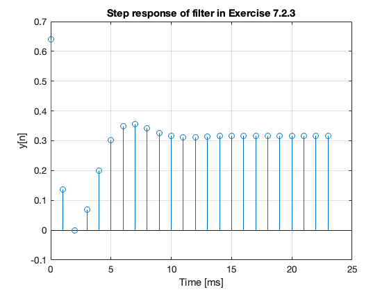
../_images/3be638b04449f56d606045cb03fcdb176dad089169012c6aaa2e9cafd7d1cd41.png

Confirm the tabulated results

yn(1:5)