Unit 7.1: Designing Analogue Filters

format compact
cd matlab

Colophon

• The source code for this page is filter_design/analogue_filters.md.

• You can view the notes for this presentation as a webpage (HTML).

• This page is downloadable as a PDF file.

Scope and Background Reading

We introduced the idea of filters in Unit 4.4: Introduction to Filters and examined in some detail the idea of an ideal low-pass filter and an approximation to the ideal filter known and the Butterworth filter. We also showed how a high-pass filter, stop-band filter and and pass-band filter could be implemented by simple manipulations of the frequency response (or transfer functions) of a low-pass filter.

An advantage of the Butterworth filter is that it has a flat response in the pass band, a consistent attenuation of -3 dB at the cut-off frequency, and a steady roll-off in the stop band. A disadvantage is that you need a high-order filter to get a fast transition between the pass-band and the stop-band.

In Example: Digital Butterworth Filter, we showed how an analogue 2nd-order Butterworth filter could be translated into a discrete-time (DT) system using the MATLAB function c2d, and we demonstrated the architecture and code that might be used to implement the digital filter.

In this unit we will explore further some of the concepts of what is called filter design by analogue prototype. This Unit is based on Chapter 11 of [Karris, 2012]. We will illustrate the concepts using MATLAB and Simulink as appropriate on the understanding that you should be able to recognize the filter type from a frequency response.

Agenda

• Introduction

• Low-pass analogue filter prototypes

  • Magnitude-square function

  • Butterworth Analogue Low-Pass Filter Design

  • Chebyshev Type I Analogue Low-Pass Filter Design

  • Chebyshev Type II Analogue Low-Pass Filter Design

  • Elliptic Analogue Low-Pass Filter Design

  • Comparison of analogue low-pass filter designs

• High-Pass, Band-Pass and Band-Elimination Filter Design

Introduction

Analogue filters are defined in continuous range of frequencies. They are classified as low-pass, high-pass, band-pass and band-elimination (band-stop) filters.

The ideal magnitude characteristics of each are illustrated in Fig. 11

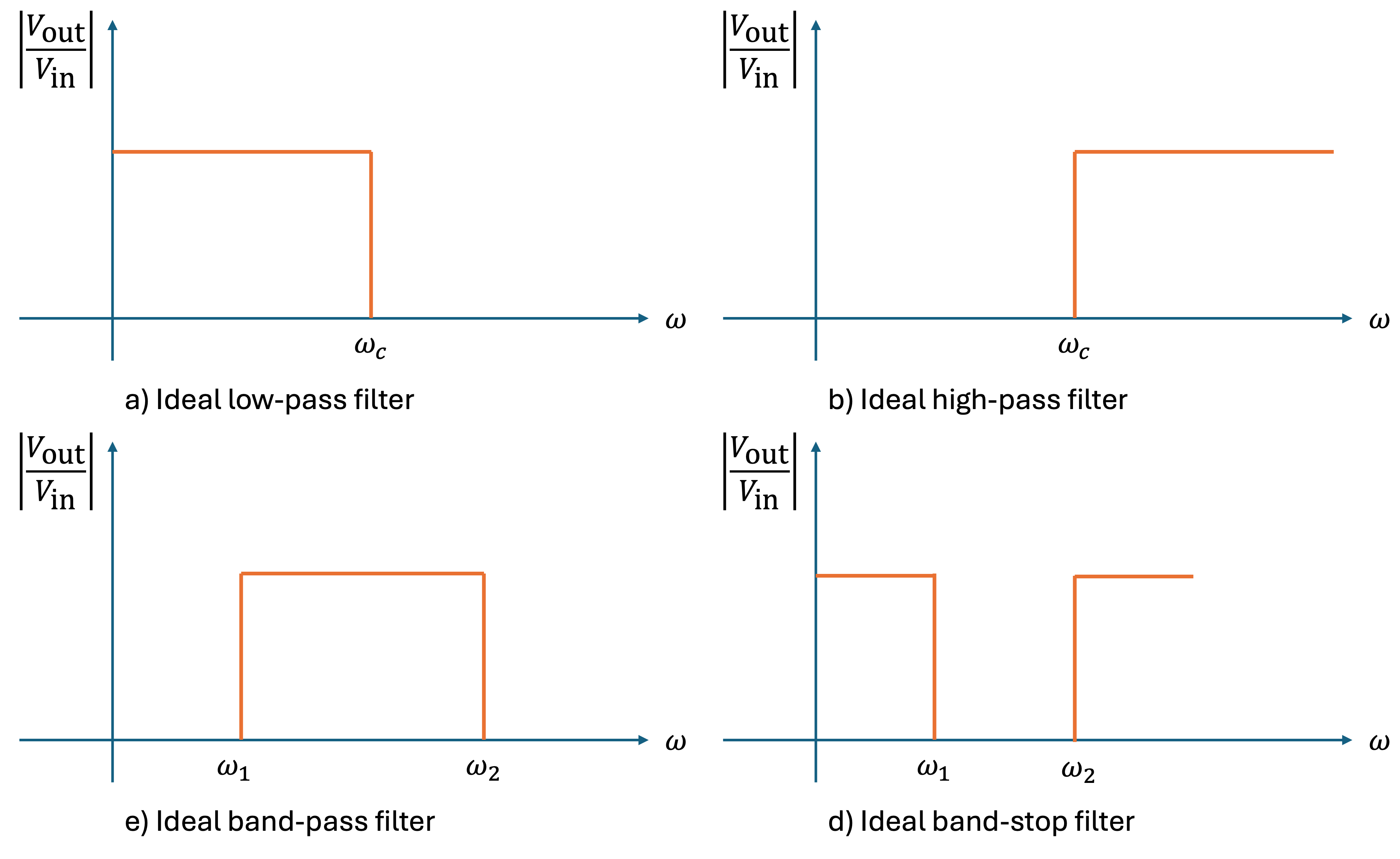
Fig. 11 Magnitude characteristics of ideal filters (reproduced from Figure 11.1 [Karris, 2012]).

As we saw in Ideal Low-Pass Filter (LPF), filters with ideal characteristics are not physically realizable (they are not causal systems). Instead we design practical filters that approximate these characteristics.

A digital filter, in general, is a computational process, or algorithm, that converts one sequence of numbers representing the input signal into another sequence of numbers representing the output signal.

Analogue filter functions have been used extensively as prototype models for designing digital filters, and that is the approach we will present here.

Note

In Section 11.2 of Karris [2012] examples of analogue low-pass and high-pass filters made from RC circuits and band-pass and stop band filters made from RLC circuits are given. We will pass over these as our interest is in digital filters, and in any case, filters made from passive components are only practical in a limited range of applications. Instead, we will look at the idea of analogue filter porotypes.

Low-pass analogue filter prototypes

In this section, we will use the analogue low-pass filter as a basis. Using transformations, we can derive high-pass and other types of filter from the low-pass filter.

We will discuss the Butterworth, Chebyshev Type I, Chebyshev Type II and Elliptic filters.

As through MATLAB and the Signal Processing Toolbox, we have access to sophisticated design tools, we will gloss over some of the mathematical details. If you are interested in such detail, please refer to Section 11.3 and following sections of [Karris, 2012].

Note

From the point of view of assessment, you are only required to be able to recognise the filter types presented here and their key properties. Although you can design a filter of virtually any order, we will limit ourselves to second-order filters and provide the actual transfer function coefficients that you need to be able to convert the analogue filter into a digital filter using the bilinear transform. If you need access to the filter formulae, you will be given them in the question.

Magnitude-square function

To facilitate the design of filters we use a so-called magnitude-squared function1 \(A^2(\omega)\), and from it derive a \(G(s)\) function such that

(16)\[A^2(\omega) = \left.G(s).G(-s)\right|_{s = j\omega}\]

Since \((j\omega)^* = (-j\omega)\), the square of a complex number can be expressed as that complex number and its complex conjugate. Thus, if the magnitude is \(A\), then

(17)\[A^2(\omega) = \left|G(j\omega)\right| = G(j\omega)G^*(j\omega) = G(j\omega).G(-j\omega)\]

Now, \(G(j\omega)\) can be considered as \(G(s)\) evaluated at \(s = j\omega\), and this (16) is justified.

Also, since \(A\) is understood to represent the magnitude, it does not need to be enclosed in vertical lines.

Not all magnitude-square functions can be decomposed to \(G(s)\) and \(G(-s)\) rational functions; only even functions of \(\omega\), positive for all \(\omega\), and proper-rational functions2 can satisfy (16).

Example 1

It is known that

\[G(s) = \frac{3s^2 + 5s + 7}{s^2 + 4s + 6} \]

Compute \(A^2(\omega)\).

Solution

Since

\[G(s) = \frac{3s^2 + 5s + 7}{s^2 + 4s + 6} \]

it follows that

\[G(-s) = \frac{3s^2 - 5s + 7}{s^2 - 4s + 6} \]

and

\[G(s).G(-s) = \frac{3s^2 + 5s + 7}{s^2 + 4s + 6}.\frac{3s^2 - 5s + 7}{s^2 - 4s + 6} = \frac{9s^4 + 17s^2 + 49}{s^4 - 4s^2 + 36} \]

Therefore

\[A^2(\omega) = \left.\frac{9s^4 + 17s^2 + 49}{s^4 - 4s^s + 36}\right|_{s = j\omega} = \frac{9\omega^4 - 17\omega^2 + 49}{\omega^4 + 4\omega^2 + 36}\]

General form of magnitude-square function

The general form of magnitude-square function \(A^2(\omega)\) is

(18)\[A^2(\omega) = \frac{C\left(b_k\omega^{2k}+b_{k-1}\omega^{2k-2}+\cdots+ b_0\right)}{a_k\omega^{2k}+a_{k-1}\omega^{2k-2}+\cdots+ a_0} \]

where \(C\) is the DC gain, \(a\) and \(b\) are constant coefficients, and \(k\) is a positive integer denoting the order of the filter.

Once the magnitude-square function \(A^2(\omega)\) is known, we can derive \(G(s)\) from (16) with the substitution \(\left(j\omega\right)^2 = -\omega^2 = - s^2\),

that is

(19)\[G(s).G(-s) = \left. A^2(\omega)\right|_{\omega^2 = -s^2}\]

Analysis of magnitude-square filter

In the simplest low-pass filter, the DC gain of the magnitude-square function is unity. In this case (18) reduces to

(20)\[A^2(\omega) = \frac{b_0}{a_k\omega^{2k}+a_{k-1}\omega^{2k-2}+\cdots+ a_0} \]

and at high frequencies (i.e. in the stop-band) can be approximated as

(21)\[A^2(\omega) = \frac{b_0/a_k}{\omega^{2k}} \]

The attenuation rate of this approximation is \(20k\) dB/decade.

Example 2

Given the magnitude-square function

(22)\[A^2(\omega) = \frac{16\left(-\omega^2 + 1\right)}{\left(\omega^2+4\right)\left(\omega^2+ 9\right)}\]

derive a suitable transfer function \(G(s)\).

Solution

From relation (19)

(23)\[G(s).G(-s) = \left. A^2(\omega)\right|_{\omega^2 = -s^2} = \frac{16\left(s^2 + 1\right)}{\left(-s^2 + 4\right)\left(-s^2 + 9\right)} \]

This function has zeros at \(s = \pm j\), and poles at \(s = \pm 2\) and \(s = \pm 3\).

There is no restriction on the zeros, but for stability3, we select the left-half \(s\)-plane poles.

Let

(24)\[G(s) = \frac{K\left(s^2 + 1\right)}{\left(s + 2\right)\left(s+3\right)} \]

We must find \(K\) such that \(G(0) = A(0)\). From (22)

\[A^2(0) = 16/36 = 4/9\]

or

\[A(0) = 2/3\]

From (24),

\[G(0) = K/6\]

and for \(G(0) = A(0)\) we must have,

\[K/6 = 2/3\]

or

\[K = 12/3 = 4\]

By subsitution into (24), we obtain

(25)\[G(s) = \frac{4\left(s^2 + 1\right)}{\left(s + 2\right)\left(s+3\right)} \]

Butterworth Analogue Low-Pass Filter Design

Consider the Butterworth low-pass filter4 whose magnitude-squared function is

(26)\[A^2(\omega) = \frac{1}{\left(\omega/\omega_c\right)^{2k}+1} \]

where \(k\) is a positive integer, and \(\omega_c\) is the cutoff (-3 dB) frequency.

We can use MATLAB to plot the frequency response of this relation for \(k = 1,2,4,8\)

w_w0 = 0:0.02:3; 
Aw2k1 = sqrt(1./(w_w0.^2 + 1)); Aw2k2 = sqrt(1./(w_w0.^4 + 1));
Aw2k4 = sqrt(1./(w_w0.^8 + 1)); Aw2k8 = sqrt(1./(w_w0.^16 + 1));
plot(w_w0,Aw2k1,w_w0,Aw2k2,w_w0,Aw2k4,w_w0,Aw2k8),grid on
xlabel('Normalized Frequency Ratio (ratio of actual to cut-off)')
ylabel('Magnitude A (square root of A^2(omega))')
title('Butterworh Analogue Low-Pass Filter characteristics for k = 1, 2, 4 and 8')
legend('k=1','k=2','k=4','k=8')

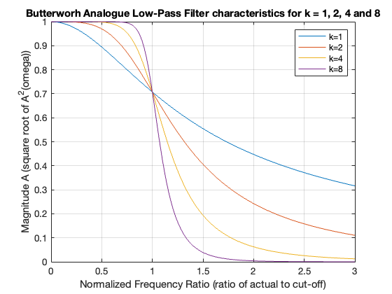
All Butterworth filters have the property that all poles of the transfer function that describes them lie on the circumference of a circle with radius \(\omega_c\), and they are \(2\pi/2k\) radians apart. Thus, if \(k\) is odd, the poles start at zero radians, and if \(k\) is even, they start at \(2\pi/2k\) radians. But regardless wether \(k\) is odd or even, the poles are distributed with symmetry with respect to the \(j\omega\) axis. For stability, we chose the left half-plave poles to form \(G(s)\).

We can find the nth roots of the complex number \(s\) by De Moirvre’s theorem. This states that

\[\sqrt[n]{r e^{j\theta}} = \sqrt[n]{r} {e}^{j\left(\frac{\theta + 2k\pi}{N} \right)}\,k=1,\pm 1,\pm 2,\ldots\]

Example 3

Derive the transfer function \(G(s)\) for the third-order (\(k=3\)) Butterworth low-pass filter with normalized cut-off frequency \(\omega_c = 1\) rad/s.

Solution

With \(k = 3\) and \(\omega_c = 1\) rad/s, (26) simplifies to

(27)\[A^2(\omega) = \frac{1}{\omega^6 + 1} \]

With the substitution \(\omega^2 = -s^2\), (26) becomes

(28)\[G(s).G(-s) = \frac{1}{-s^6 + 1} \]

The poles of (28) are given by \(\left(1 - s^6\right) = 0\) or \(s = \sqrt[6]{1}\).

That is, \(s = \sqrt[6]{1}\angle 0 ^\circ\) and, by De Moivre’s theorem, with \(n = 6\),

\[\sqrt[6]{1e^{j0}} = \sqrt[6]{1}e^{j\left(\frac{0 + 2k\pi}{6} \right)},\,k=0,1,2,3,4,5\]

Thus

\[\begin{split} \begin{array}{lll} s_1 = 1\angle 0^\circ & s_2 = 1\angle 60^\circ = \frac{1}{2} + j\frac{\sqrt{3}}{2} & s_3 = 1\angle 120^\circ = -\frac{1}{2} + j\frac{\sqrt{3}}{2} \\ s_4 = 1\angle 180^\circ = -1 & s_5 = 1\angle 240^\circ = -\frac{1}{2} - j\frac{\sqrt{3}}{2} & s_6 = 1\angle 300^\circ = \frac{1}{2} - j\frac{\sqrt{3}}{2} \end{array} \end{split}\]

As expected, these six poles lie on the circumference of the circle with radius \(\omega_c = 1\) as shown in Fig. 12.

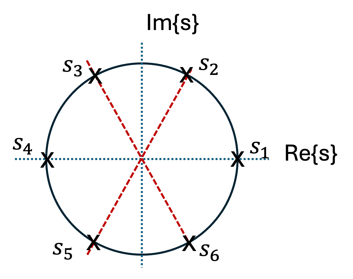
Fig. 12 Location of the poles for the transfer function for the transfer function of Example 3

The transfer function \(G(s)\) is formed with the left half-plane poles \(s_3\), \(s_4\) and \(s_5\). Then

(29)\[G(s) = \frac{K}{\left(s + 1\right)\left(s + \frac{1}{2} -j\frac{\sqrt{3}}{2}\right)\left(s + \frac{1}{2} +j\frac{\sqrt{3}}{2}\right)} \]

We use MATLAB to express the denominator as a polynomial

syms s; den = (s + 1)*(s + 1/2 - j*sqrt(3)/2)*(s + 1/2 + j*sqrt(3)/2)

den =

(s + 1)*(s - (3^(1/2)*1i)/2 + 1/2)*(s + (3^(1/2)*1i)/2 + 1/2)

expand(den)

ans =

s^3 + 2*s^2 + 2*s + 1

Therefore (28) simplifies to

(30)\[G(s) = \frac{K}{s^3 + 2s^2 + 2s + 1} \]

The gain \(K\) is found from \(A^2(0) = 1\) and \(G(0) = K\). Thus, K = 1 and

(33)\[G(s) = \frac{1}{s^3 + 2s^2 + 2s + 1} \]

The generalized form of any analogue low-pass filter (Butterworth, Chebyshev, Elliptic, etc) is

(34)\[\left.G(s)\right|_{\mathrm{lp}} = \frac{b_0}{a_ks^k + \cdots a_2 s^2 + a_1 s + a_0} \]

The pole locations and coefficients of the corresponding denominator polynomials have been derived and tabulated and easily found on the internet: for example Normalized Butterworth polynomials in Wikipedia.

For brevity, we will not reproduce these tables here.

Designing Butterworth filters in MATLAB

The MATLAB functions buttap and zp2tf can also be used to derive the coefficients.

The buttap function returns the zeros, poles and gain for an Nth order normalized prototyoe Butterworth low-pass filter. The resulting filter has \(N\) poles around the unit circle in the left half plane, and no zeros. The zp2tf function performs the zero-pole-gain to transfer function conversion.

Example 4

Use MATLAB to derive the numerator b and denominator a coefficients for the third-order Butterworth low-pass filter prototype with normalized cutoff frequency. Plot the Bode plot of the filter.

Solution

[z,p,k] = buttap(3); 
[b,a] = zp2tf(z,p,k)

b =
         0         0         0    1.0000

a =
    1.0000    2.0000    2.0000    1.0000

G = tf(b,a)
bode(G), grid on
title('Bode diagram for a 3rd order Butterworth filter with wc = 1 rad/s')

G =

            1

  ---------------------

  s^3 + 2 s^2 + 2 s + 1

Continuous-time transfer function.

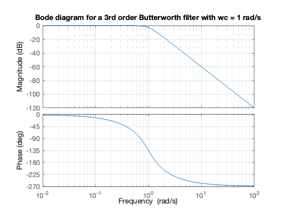
Note that the roll-off is -60 dB/decade above the normalized cut-off \(\omega_c = 1\) rad/s. Also note that the phase changes fron \(0^\circ\) to \(-270^\circ\) from low to high frequency.

Denormalizing a prototype filter

The examples given so far, and the MATLAB function buttap (and the others we will meet later) give the coefficents assuming that the cut-off frequency \(\omega_c\) is 1 rad/s. To denormalize the filter coefficients, we need to change the radius of the circle shown e.g in Fig. 12 from \(\omega_c = 1\) to \(\omega_c = \omega_\mathrm{actual}\) .

To do this we make the subsitution

(33)\[G(s)_\mathrm{actual} = G\left(\frac{s}{\omega_\mathrm{actual}} \right) \]

As you might expect, MATLAB provides a function for that: lp2lp.

Example 5

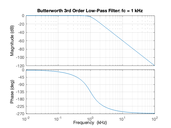
Redesign the filter designed in Example 4 so that it has a a cut-off frequency of \(1\) kHz.

Solution

[z,p,k] = buttap(3); 
[b,a] = zp2tf(z,p,k);
fc = 1e3; % 1 kHz
wc = 2*pi*fc; % rad/s
format long
[b, a] = lp2lp(b, a, wc)

b =
     2.480502134423985e+11

a =
   1.0e+11 *
  Columns 1 through 3
   0.000000000010000   0.000000125663706   0.000789568352087
  Column 4
   2.480502134423986

h = bodeplot(tf(b, a)); setoptions(h,'FreqUnits','kHz'),grid on
title('Butterworth 3rd Order Low-Pass Filter: fc = 1 kHz')

Defining the stop-band attenuation in a Butterworth filter

Quite often, we require that in the stop-band of the filter, that is when \(\omega \ge \omega_c\), the attenuation is larger than \(-20\) dB/decade. That is, we require a sharper cut-off. As can be seen from the plots of Butterworth Analogue Low-Pass Filter Design, the Butterworth becomes sharper for larger values of \(k\). To see this more clearly, we generate a family of attenuation curves using the MATLAB script given below:

w_w0 = 1:0.01:10; dBk1 = 20.*log10(sqrt(1./(w_w0.^2 + 1)));
dBk2 = 20.*log10(sqrt(1./(w_w0.^4 + 1))); dBk3 = 20.*log10(sqrt(1./(w_w0.^6 + 1)));
dBk4 = 20.*log10(sqrt(1./(w_w0.^8 + 1))); dBk5 = 20.*log10(sqrt(1./(w_w0.^10 + 1)));
dBk6 = 20.*log10(sqrt(1./(w_w0.^12 + 1))); dBk7 = 20.*log10(sqrt(1./(w_w0.^14 + 1)));
dBk8 = 20.*log10(sqrt(1./(w_w0.^16 + 1)));
semilogx(w_w0,dBk1,w_w0,dBk2,w_w0,dBk3,w_w0,dBk4,...
         w_w0,dBk5,w_w0,dBk6,w_w0,dBk7,w_w0,dBk8)
xlabel('Normalized Frequency (rad/sec)'),ylabel('Magnitude Response (dB)')
title('Magnitude Attenuation ad a Fuction of Noramized Frequency')
set(gca, 'XTick',[1:10]),grid
legend('k = 1','k = 2','k = 3','k = 4','k = 5','k = 6','k = 7','k = 8')

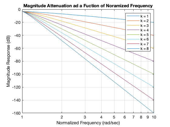
This plot indicates that for \(k = 1\) the attenuation is \(-20\) dB/decade, for \(k=2\), the attenuation is \(-40\) dB/decade, and so on. In general, the attenuation is \(-20k\) dB/decade for a Butterworth filter.

Note

We have used several new MATLAB commands in Example 5. These are summarized below.

• lp2lp - change cutoff frequency for lowpass analogue filter.

• bodeplot - plot Bode frequency response with additional plot customization options.

• option FreqUnits - changes the units for frequency response data.

Karris [2012] goes on to give more details of the Butterworth filter, including how to chose the filter order \(N\) to match a specific requirement on the stop-band attenuation, and how such a filter might be implemented with Op-Amp circuits. We leave you to explore these topics on your own.

Chebyshev Type I Analogue Low-Pass Filter Design

An issue with the Butterworth filter is that the stop-band attenuation rate may not be high enough for some applications unless a very large value of \(N\) is used.

If we allow some ripple in the pass-band we can obtain a sharper cut-off for smaller values of \(N\).

The Chebyshev analogue low-pass filter is such a design.

The model transfer function for a Type I Chebyshev filter is

(34)\[ A^2(\omega) = \frac{\alpha}{1 + \epsilon^2C_k^2(\omega/\omega_c)} \]

Where \(C_k\) is the Chebyshev polynomial5 of degree \(k\), and \(\epsilon^2\) is a parameter that is used to set the pass-band ripple.

A Chebyshev filter has the same transfer function structure as (34), but the poles are located on an elipse rather than a circle.

We will not present the formulae used to define the poles of this filter type, as MATLAB provides the design tool cheb1ap that will do this for us.

Example 6

Use the MATLAB function cheb1ap to design a second-order Chebysehv Type I low-pass filter with 3 dB ripple in the pass-band.

Solution

The cheb1ap function takes two arguments, the order \(N\) and the pass-band ripple (in dB). It returns the zero-pole-gain values as vectors.

To solve the problem, we use the script:

w = 0:0.05:400; % Range of frequencies to plot.
[z,p,k] = cheb1ap(2, 3);
[b, a] = zp2tf(z, p, k) % Convert zeros and poles of G(s) to polynomial form

b =
                   0                   0   0.501188646503800

a =
   1.000000000000000   0.644899651302867   0.707947780125280

Now, with the known values of a and b, we can use the bode function to produce the magnitude and phase plots as follows.

bode(b, a)
title('Bode plot for Type | Second-Order Chebyshev Low-Pass Filter')
grid on

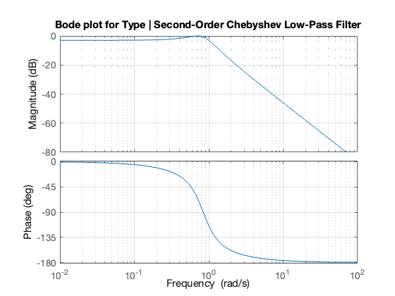
On the Bode plots shown, the ripple is not so obvious. The reason is that the Magnitude is in dB so the plot is essentially a linear approximation. To see the ripple we plot magnitude:

w = 0:0.01:10; 
Gs = freqs(b, a, w); % returns response as complex values
semilogx(w,abs(Gs)),grid on
xlabel('Frequency in rad/s'),ylabel('Magnitude of G(s)')
title('Type I Chebyshev Low-Pass Filter')

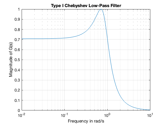
The function freqs computes the complex frequency response \(H(j\omega)\) of an analogue filter \(H(s) = b(s)/a(s)\).

Chebyshev Type II Analogue Low-Pass Filter Design

A Type II Chebyshev filter has ripple in the stop-band. It is defined by the magnitude squared expression:

(35)\[ A^2(\omega) = \frac{\epsilon^2C_k^2(\omega/\omega_c)}{1 + \epsilon^2C_k^2(\omega/\omega_c)} \]

We can design Chebyshev Type II low-pass filters with the MATLAB cheb2ap function.

Example 7

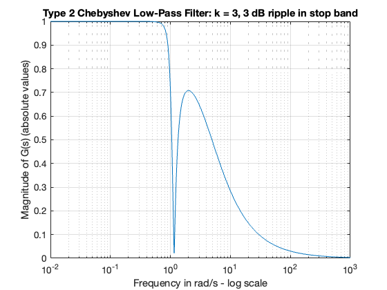
Using the MATLAB cheb2ap function, design a third-order Chebyshev analogue filter with 3 dB ripple in the stop band.

Solution

We begin with the MATLAB script reporoduced below.

w = 0:0.01:1000; 
[z,p,k] = cheb2ap(3,3);
[b, a] = zp2tf(z,p,k)

b =
  Columns 1 through 3
                   0   3.007131879022801                   0
  Column 4
   4.009509172030401

a =
  Columns 1 through 3
   1.000000000000000   3.716637149027132   2.385274779846660
  Column 4
   4.009509172030401

Plot this response

Gs = freqs(b, a, w); semilogx(w,abs(Gs))
xlabel('Frequency in rad/s - log scale')
ylabel('Magnitude of G(s) (absolute values)')
title('Type 2 Chebyshev Low-Pass Filter: k = 3, 3 dB ripple in stop band')
grid

Elliptic Analogue Low-Pass Filter Design

The elliptic filter, also known as Cauer filter, is characterized by the low-pass magnutude-squared function

(36)\[ A^2(\omega) = \frac{1}{1 + R_k^2\left(\omega/\omega_c\right)} \]

where \(R_k(x)\) represents a rational elliptic function used with eliptic integrals.

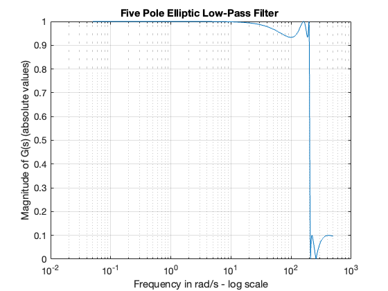
Elliptic filters have ripple in both the pass-bad and stop-band, but have a very steep transiition between these bands.

We can design elliptic low-pass filters with the ellip function. The statement

[z,p,k] = ellip(N,Rp,Rs,W0,'s')

returns the pole-zero-gain values for an elliptic low-pass filter of order N, with a maximum passband ripple of Rp dB, a stop-band ripple of Rs dB, cut-off frequency of W0 rad/s. The argument ‘s’ returns the poles and zeros of an analogue filter. If ommitted, the function designs a discrete-time filter.

Example 8

Use the MATLAB function ellip to design a fifth-order analogue eliptic low-pass filter with \(\omega_c = 200\) rad/s, pass-band ripple of \(0.6\) dB and stop-band ripple of \(20\) dB. Plot the magnitude frequency response of the filter.

Solution

w = 0:0.05:500;
[z,p,k] = ellip(5, 0.6, 20, 200, 's');
[b,a] = zp2tf(z,p,k);

Gs = freqs(b,a,w);
semilogx(w,abs(Gs)),grid on
xlabel('Frequency in rad/s - log scale'),ylabel('Magnitude of G(s) (absolute values)')
title('Five Pole Elliptic Low-Pass Filter ')

Comparison of analogue low-pass filter designs

Figure Fig. 13 shows the Butterworth, Chebyshev and Elliptic filters for a fifth-order prototype analogue low-pass filter.

Fig. 13 Frequency response curves of four linear analog filters: Butterworth filter, Chebyshev filter of type 1 and 2 and Elliptic filter, each one as 5th order filter. (Originally published as Filters_order5.svg on WikiPedia article Chebyshev filter. Image CC BY Geek2)

As you can see, the Chebyshev filters are sharper than the Butterworth filter; they are not as sharp as the elliptic one, but they show fewer ripples over the bandwidth.

Advantages and disadvantages of different types of filters

Filter Type	Advantages	Disadvantages
Butterworth	Simplest design; Flat pass band	Slow rate of attenuation for order 4 or less
Chebyshev Type I	Sharp cuttoff rate in transition (pass to stop) band	Ripple in pass band. Bad (non-linear) phase response
Chebyshev Type II	Sharp cuttoff rate in transition (pass to stop) band	Ripple in stop band. Bad (non-linear) phase response
Elliptic (Cauer)	Sharpest cutoff rate among all other types of filters	Ripple in both pass and stop band. Worst (most non-linear) phase response among the other types of filters.

High-Pass, Band-Pass and Band-Elimination Filter Design

Prototype analogue filters can be converted to high-pass, band-pass and band-elimination (band-stop filters) by the application of frequency transformations on \(s\) in \(G(s)\). These transformations are listed in Table 11.5 on Page 11-40 of [Karris, 2012] and will not be reproduced here. Instead we will introduce the MATLAB transformation functions and give some examples of their use.

Low-pass to low-pass

As already seen in Denormalizing a prototype filter, the function lp2lp will convert a normalised low-pass analogue filter with cut-off frequency \(\omega_c = 1\) to \(\omega_c = \omega_\mathrm{actual}\).

See Denormalizing a prototype filter for an example.

Low-pass to high-pass

The MATLAB function lp2hp will convert a low-pass analogue filter to a high-pass analogue filter.

Example 9

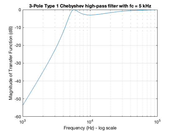
Use the MATLAB commands cheb1ap and lp2hp to derive the transfer function of a 3-pole Chebyshev Type I analogue high-pass filter with cutoff frequency \(f_c = 5\) kHz.

Solution

We will use the cheb1ap command to derive the transfer function \(G(s)\) of the low-pass filter with normalized cutoff frequency at \(\omega_c = 1\) rad/s. Then we will use the command lp2hp to transform \(G(s)\) to another transfer function \(G'(s)\) with cut-off frequency at \(f_c = 5\) kHz or \(\omega_c = 2\pi\times 5\times 10^3\) rad/s.

% design 3 pole Type I Chebyshev low-pass filter, wc = 1 rad/s
[z,p,k] = cheb1ap(3,3);    % 3 pole, 3dB ripple in pass band
[b,a] = zp2tf(z,p,k);      % Compute numerator and denoninator coefficents with wcn = 1 rad/s
f = 1000:100:100000;       % Define frequency range to plot
fc = 5000;                 % Define actual cutoff frequency at 5 kHz
wc = 2*pi*fc;              % Convert desired cut-off frequency to rad/s       
[bn,an] = lp2hp(b, a, wc); % Compute numerator and denoninator coefficents of high-pass filter with fc = 5 kHz

% Compute and plot frequency response of high-pass filter
Gsn = freqs(bn, an, 2*pi*f);
semilogx(f, 20*log10(abs(Gsn))), grid
xlabel('Frequency (Hz) - log scale'),ylabel('Magnitude of Transfer Function (dB)')
title('3-Pole Type 1 Chebyshev high-pass filter with fc = 5 kHz')

Low-pass to band-pass

The MATLAB function lp2bp will convert a normalized low-pass analogue filter to a band-pass analogue filter.

Example 10

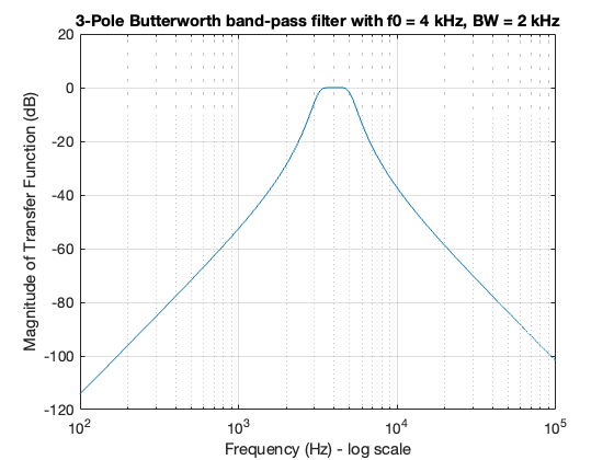
Use the MATLAB commands buttap and lp2bp to derive the transfer function of a 3-pole Butterworth analogue band-pass filter with the pass band frequency centred at \(f_0 = 4\) kHz, and bandwidth \(\mathrm{BW} = 2\) kHz.

Solution

We will use the buttap function to derive the transfer function \(G(s)\) of the low-pass analogue filter with normalized cutoff frequency at \(\omega_c = 1\) rad/s. Then we will use the command lp2bp to transform \(G(s)\) to another transfer function \(G'(s)\) with centred frequency at \(f_0 = 4\) kHz and bandwith \(\mathrm{BW} = 2\) hHz.

format short;
% design 3 pole Butterworth low-pass filter, wc = 1 rad/s
[z,p,k] = buttap(3);       % 3 pole
[b,a] = zp2tf(z,p,k);      % Compute numerator and denoninator coefficents with wcn = 1 rad/s
f = 100:100:100000;        % Define frequency range to plot
f0 = 4000;                 % Define center frequency at 4 kHz
W0 = 2*pi*f0;              % Convert desired centre frequency to rad/s    
fbw = 2000;                % Define bandwidth
Bw = 2*pi*fbw;             % Convert desired bandwidth to rad/s
[bn,an] = lp2bp(b, a, W0, Bw); % Compute numerator and denoninator coefficents of band-pass filter

% Compute and plot frequency response of band-pass filter
Gsn = freqs(bn, an, 2*pi*f);
semilogx(f, 20*log10(abs(Gsn))), grid
xlabel('Frequency (Hz) - log scale'),ylabel('Magnitude of Transfer Function (dB)')
title('3-Pole Butterworth band-pass filter with f0 = 4 kHz, BW = 2 kHz')

Low-pass to band-stop

The MATLAB function lp2bs will convert a low-pass normalized analogue filter to a band-stop analogue filter.

Example 11

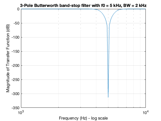
Use the MATLAB commands buttap and lp2bs to derive the transfer function of a 3-pole Butterworth analogue band-elimination (band-stop) filter with the stop band frequency centred at \(f_0 = 5\) kHz, and bandwidth \(\mathrm{BW} = 2\) kHz.

Low-pass to band-pass

The MATLAB function lp2bp will convert a low-pass filter to a band-pass filter.

Solution

We will use the buttap function to derive the transfer function \(G(s)\) of the low-pass analogue filter with normalized cutoff frequency at \(\omega_c = 1\) rad/s. Then we will use the command lp2bs to transform \(G(s)\) to another transfer function \(G'(s)\) with centred frequency at \(f_0 = 5\) kHz and bandwith \(\mathrm{BW} = 2\) hHz.

format short;
% design 3 pole Butterworth low-pass filter, wc = 1 rad/s
[z,p,k] = buttap(3);       % 3 pole
[b,a] = zp2tf(z,p,k);      % Compute numerator and denoninator coefficents with wcn = 1 rad/s
f = 1000:100:10000;        % Define frequency range to plot
f0 = 5000;                 % Define center frequency at 4 kHz
W0 = 2*pi*f0;              % Convert desired centre frequency to rad/s    
fbw = 2000;                % Define bandwidth
Bw = 2*pi*fbw;             % Convert desired bandwidth to rad/s
[bn,an] = lp2bs(b, a, W0, Bw); % Compute numerator and denoninator coefficents of band-pass filter

% Compute and plot frequency response of band-pass filter
Gsn = freqs(bn, an, 2*pi*f);
semilogx(f, 20*log10(abs(Gsn))), grid
xlabel('Frequency (Hz) - log scale'),ylabel('Magnitude of Transfer Function (dB)')
title('3-Pole Butterworth band-stop filter with f0 = 5 kHz, BW = 2 kHz')

Unit 7.1 Summary

In this unit we have looked at the design of prototype analogue low-pass filters which is a basis for filter design in general. We have demonstrated how the analogue-squared function \(A^2(\omega) = G(s)G(-s)\) can be used to design an analogue filter \(G(s)\) with particular properties, we then looked at the Butterworth filter, Chebyshev Type I and Type II filters and the elliptic filter. We explored the MATLAB tools provided by the Signal Processing Toolbox that can used to these design these prototype filters and the functions that can be used to denormalize the cutoff frequency and design high-pass, band-pass and band-stop filters.

These are the topics we covered:

• Introduction

• Low-pass analogue filter prototypes

  • Magnitude-square function

  • Butterworth Analogue Low-Pass Filter Design

  • Chebyshev Type I Analogue Low-Pass Filter Design

  • Chebyshev Type II Analogue Low-Pass Filter Design

  • Elliptic Analogue Low-Pass Filter Design

  • Comparison of analogue low-pass filter designs

• High-Pass, Band-Pass and Band-Elimination Filter Design

Unit 7.1 Takeaways

Coming Next

We will conclude this module in Unit 7.1: Designing Analogue Filters with a look at how analogue prototype filters can be digitized, how the digitized filters can be implemented and a demonstration of the interactive filter-design tools provided by MATLAB.

MATLAB functions introduced in Unit 7.1

Analogue prototype designers

Used to design an analogue prototype low-pass filter \(G(s)\) with normalized cutoff frequency \(\omega_c = 1\) rad/s. The examples in this unit show the functions returning the zeros, poles and gain of the equivalent transfer function \(G(s)\). They can all return the numerator and denominator polynomial coeffiecients of \(G(s) = b(s)/a(s)\) directly.

• buttap - \(N\)-pole Butterworth analogue prototype low-pass filter.

• cheb1ap - \(N\)-pole Chebyshev Type I analogue prototype low-pass filter with defined pass-band ripple.

• cheb2ap - \(N\)-pole Chebyshev Type II analogue prototype low-pass filter with defined stop-band ripple.

• ellipap - \(N\)-pole Elliptic analogue prototype low-pass filter with defined pass-band and stop-band ripple.

Filter transformation functions

These functions convert the analogue low-pass filter \(G(s)\) with normalized cutoff frequency \(\omega_c = 1\) \rad/s and convert it to a new filter \(G'(s)\).

• lp2lp - converts an analogue low-pass filter with \(\omega_c = 1\) to one with \(\omega_c = \omega_\mathrm{actual}\).

• lp2hp - converts an analogue low-pass filter with \(\omega_c = 1\) to a high-pass filter with \(\omega_c = \omega_\mathrm{actual}\).

• lp2bp - converts an analogue low-pass filter with \(\omega_c = 1\) to a band-pass filter with defined centre frequency \(f_0\) and bandwidth \(\mathrm{BW}\).

• lp2lp - converts an analogue low-pass filter with \(\omega_c = 1\) to a band-stop filter with defined centre frequency \(f_0\) and bandwidth \(\mathrm{BW}\).

Utility functions

• zp2tf - return the numerator and denominator polynomial coeffiecients of \(G(s) = b(s)/a(s)\) from the zeros, poles and gain returned by the design functions.

• fregs - return the CT frequency response of an analogue filter

• semilogx - plot y against the log of x.

• tf - create an LTI system object

• bode - Bode ploto of an LTI system: magnitude in dB, phase in degrees plotted against log frequency.

• mag2db - Converts magnitude into dB using \(20\log_{10} M\).

References

See Bibliography.

Footnotes

---

1

This avoids having to deal with complex magnitudes which use the square-root operator.

2

A rational function is said to be proper if the largest power in the denominator is equal to or larger than that of the numerator.

3

A system is said to be stable if a finite input produces a finite output. Alternatively, a system is stable if its impulse response \(h(t)\) vanishes after a sufficiently long time. For linear time-invariant systems, a system will be stable only if all the real-parts of the poles have negative sign. That is, they lie in the left-half of the \(s\)-plane.

4

The frequency response of the Butterworth filter is maximally flat (has no ripples) in the passband, and rolls off towards zero in the stopband. When viewed on a logarithmic Bode plot, the response slopes off linearly at a rate of \(-20k\) dB/decade towards negative infinity.

5

The derivation of the Chebyshev polynomials is outside the scope of this unit, but if you are interested you can review one of the many online resources: e.g. Chebyshev polynomials [WikiPedia]. The Chebyshev polynomials of the first kind are used in the design of filters. If you want the details, please consult Section 11.2.2 of Karris [2012]. See also Chebyshev filter [WikiPedia]