System response from the system impulse response#

Recall that the convolution integral of a system with impulse response $h(t)$ and input $u(t)$ is

We let

Then by the time convolution property

The System Function#

We call $H(\omega )$ the system function.

We note that the system function $H(\omega )$ and the impulse response $h(t)$ form the Fourier transform pair

Obtaining system response#

If we know the impulse resonse $h(t)$, we can compute the system response $g(t)$ of any input $u(t)$ by multiplying the Fourier transforms of $H(\omega )$ and $U(\omega )$ to obtain $G(\omega )$. Then we take the inverse Fourier transform of $G(\omega )$ to obtain the response $g(t)$.

1. Transform $h(t)\to H(\omega )$

2. Transform $u(t)\to U(\omega )$

3. Compute $G(\omega )=H(\omega ).U(\omega )$

4. Find ${\mathcal{F}}^{-1}\{G(\omega )\}\to g(t)$

Example 1#

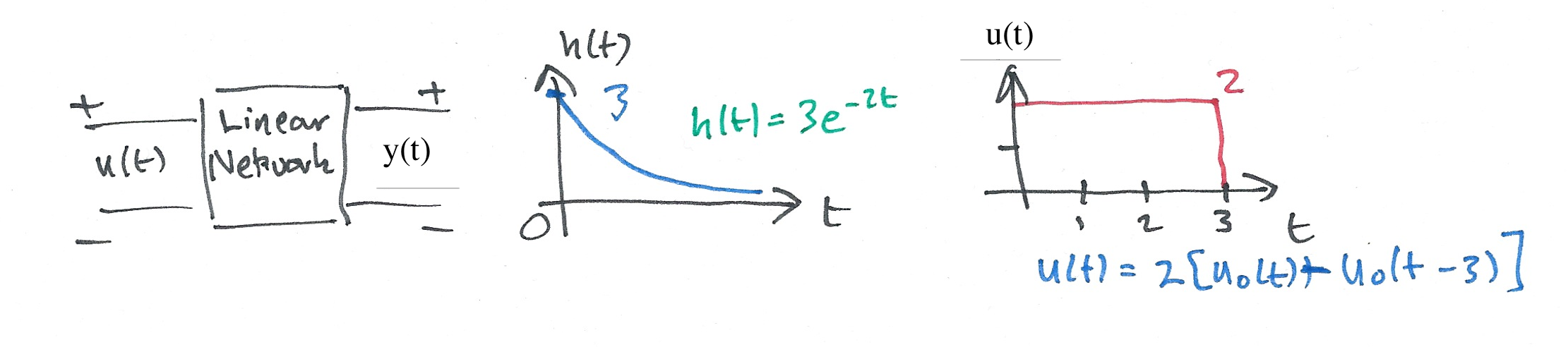
Karris example 8.8: for the linear network shown below, the impulse response is $h(t)=3e^{-2t}{u}_0(t)$. Use the Fourier transform to compute the response $y(t)$ when the input $u(t)=2[u_0(t)-u_0(t-3)]$. Verify the result with MATLAB.

Solutions see: Worked Solutions

MATLAB verification of example 1#

format compact; % reduce whitesace for textbook presentation
syms t w
U1 = fourier(2*heaviside(t),t,w)

U1 =
2*pi*dirac(w) - 2i/w

H = fourier(3*exp(-2*t)*heaviside(t),t,w)

H =
3/(2 + w*1i)

Y1=simplify(H*U1)

Y1 =
3*pi*dirac(w) - 6i/(w*(2 + w*1i))

y1 = simplify(ifourier(Y1,w,t))

y1 =
(3*exp(-2*t)*(sign(t) + 1)*(exp(2*t) - 1))/2

Get y2

Substitute $t-3$ into $t$.

y2 = subs(y1,t,t-3)

y2 =
(3*exp(6 - 2*t)*(sign(t - 3) + 1)*(exp(2*t - 6) - 1))/2

y = y1 - y2

y =
(3*exp(-2*t)*(sign(t) + 1)*(exp(2*t) - 1))/2 - (3*exp(6 - 2*t)*(sign(t - 3) + 1)*(exp(2*t - 6) - 1))/2

The result is equivalent to:

y = 3*heaviside(t) - 3*heaviside(t - 3) + 3*heaviside(t - 3)*exp(6 - 2*t) - 3*exp(-2*t)*heaviside(t)

Which after gathering terms gives

$$y(t)=3(1-3e^{-2t})u_0(t)-3(1-3e^{-2(t-3)})u_0(t-3)$$

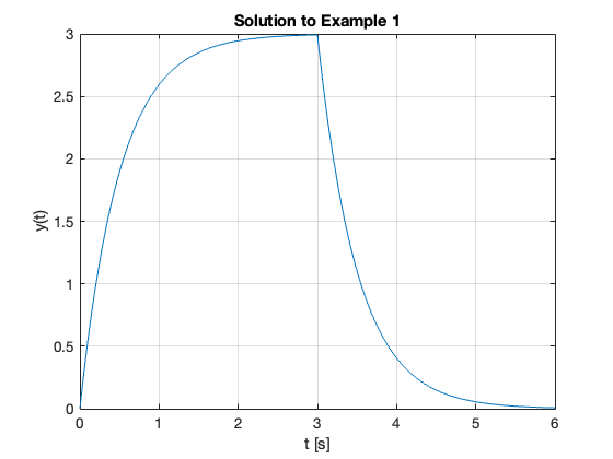
Plot result

fplot(y,[0,6])
title('Solution to Example 1')
ylabel('y(t)')
xlabel('t [s]')
grid 

Example 2#

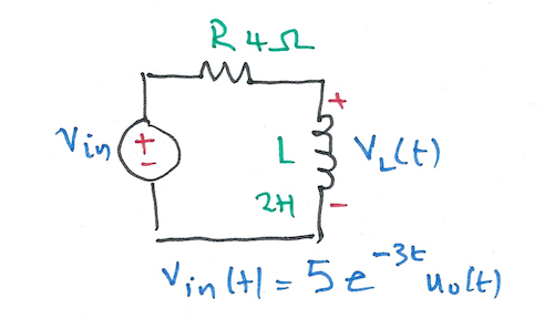
Karris example 8.9: for the circuit shown below, use the Fourier transfrom method, and the system function $H(\omega )$ to compute $V_L(t)$. Assume $i_L(0^{-})=0$. Verify the result with Matlab.

MATLAB verification of example 2#

syms t w
H = j*w/(j*w + 2)

H =
(w*1i)/(2 + w*1i)

Vin = fourier(5*exp(-3*t)*heaviside(t),t,w)

Vin =
5/(3 + w*1i)

V_L=simplify(H*Vin)

V_L =
(w*5i)/((2 + w*1i)*(3 + w*1i))

v_L = simplify(ifourier(V_L,w,t))

v_L =
-(5*exp(-3*t)*(sign(t) + 1)*(2*exp(t) - 3))/2

The result is equivalent to:

vout = -5*exp(-3*t)*heaviside(t)*(2*exp(t) - 3)

Which after gathering terms gives

$$v_{\mathrm{out}}=5(3e^{-3t}-2e^{-2t})u_0(t)$$

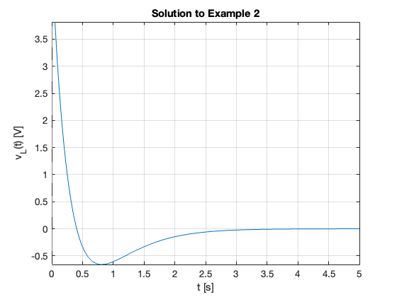
Plot result

fplot(v_L,[0,5])
title('Solution to Example 2')
ylabel('v_L(t) [V]')
xlabel('t [s]')
grid 

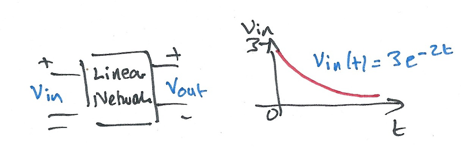
Example 3#

Karris example 8.10: for the linear network shown below, the input-output relationship is:

where $v_{\mathrm{in}}=3e^{-2t}$. Use the Fourier transform method, and the system function $H(\omega )$ to compute the output $v_{\mathrm{out}}$. Verify the result with Matlab.

Matlab verification of example 3#

syms t w
H = 10/(j*w + 4)

H =
10/(4 + w*1i)

Vin = fourier(3*exp(-2*t)*heaviside(t),t,w)

Vin =
3/(2 + w*1i)

Vout=simplify(H*Vin)

Vout =
30/((2 + w*1i)*(4 + w*1i))

vout = simplify(ifourier(Vout,w,t))

vout =
(15*exp(-4*t)*(sign(t) + 1)*(exp(2*t) - 1))/2

The result is equiavlent to:

15*exp(-4*t)*heaviside(t)*(exp(2*t) - 1)

Which after gathering terms gives

$$v_{\mathrm{out}}(t)=15(e^{-2t}-e^{-4t})u_0(t)$$

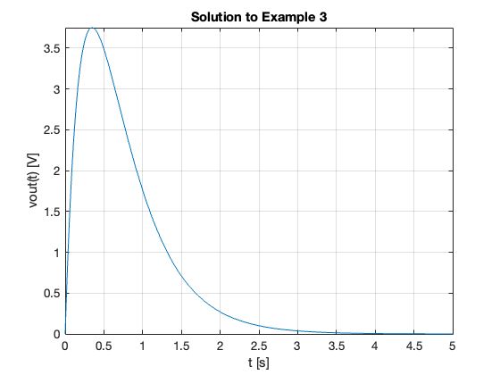
Plot result

fplot(vout,[0,5])
title('Solution to Example 3')
ylabel('vout(t) [V]')
xlabel('t [s]')
grid 

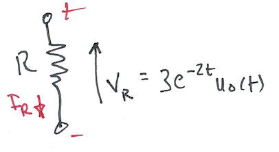
Example 4#

Karris example 8.11: the voltage across a 1 $\mathrm{\Omega }$ resistor is known to be $V_R(t)=3e^{-2t}{u}_0(t)$. Compute the energy dissipated in the resistor for $0<t<\mathrm{\infty }$, and verify the result using Parseval’s theorem. Verify the result with Matlab.

Note from tables of integrals

syms t w

Vr = 3*exp(-2*t)*heaviside(t);
R = 1;
Pr = Vr^2/R
Wr = int(Pr,t,0,inf)
double(Wr)

Pr =
9*exp(-4*t)*heaviside(t)^2
Wr =
9/4
ans =
    2.2500

Fw = fourier(Vr,t,w)

Fw =
3/(2 + w*1i)

Fw2 = simplify(abs(Fw)^2)

Fw2 =
9/abs(2 + w*1i)^2

Wr=2/(2*pi)*int(Fw2,w,0,inf)
double(Wr)

Wr =
(51607450253003931*pi)/72057594037927936
Wr =
    2.2500