Unit 3.3: Computing Line Spectra#
In Unit 3.2: Exponential Fourier Series we saw that we could exploit the complex exponential \(e^{j\omega t}\) to redefine trigonometric Fourier series into the exponential Fourier series and in so doing we eliminate one integration and at the same time simplify the calculation of the coefficients of the Fourier series.
In this section we show how the exponential form of the Fourier series leads us to the ability to present waveforms as line spectra which simplifies the calculation of power for systems with harmonics and leads in the limit as 𝑇 approaches infinity to the Fourier Transform.
Colophon#
An annotatable worksheet for this presentation is available as Worksheet 4.
The source code for this page is fourier_series/3/exp_fs2.md.
You can view the notes for this presentation as a webpage (Unit 3.3: Computing Line Spectra).
This page is downloadable as a PDF file.
Agenda#
Fundamental frequency#
Fundamental frequency – A periodic signal \(f(t) = f(t + nT),\; n\in \mathbb{Z}\) has period \(T\) s and a fundamental frequency \(f_0 = 1/T\) Hz.
When used in Fourier series and Fourier transforms, frequencies are expressed as \(\omega\) in radians/second.
The fundamental frequency is \(\omega = \Omega_0 = 2 \pi f_0\) or, equivalently, \(\Omega_0 = 2 \pi /T\) rad/s.
Harmonic frequencies#
Harmonic frequencies (or harmonics) are simply integer multiples of the fundamental frequency \(\Omega_0\).
The zero-th harmonic is \(\Omega_0 = 0\) rad/s or DC.
The first harmonic is \(1.\Omega_0 = \Omega_0\), is the fundamental frequency,
The second harmonic is \(2 \Omega_0\),
The third harmonic is \(3 \Omega_0\), etc.
In general, we can express the \(k\)-th harmonic as \(k\Omega_0,\; k\in \mathbb{Z}\).
Line Spectra#
The use of line spectra diagrams is a useful way to visualize the harmonic frequency components of a peiodic signal.
In MATLAB, the easiest way to plot this is using a stem plot of the lines, representing the Fourier series (FS) coefficients, plotted against \(k\).
Line Spectra for Exp. FS#
When the exponential Fourier series are known it is useful to plot the amplitude and phase of the harmonics on a frequency scale.
This is the spectrum of the Exponential Fourier Series calculated in Computing coefficients of Exponential Fourier Series in MATLAB is reproduced in fig:5.3.1
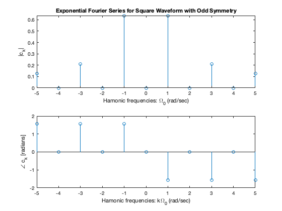
Fig. 2 Exponential Fourier Series spectrum for the square wave calculated in fs2:eg.#
Line Spectra for Trig. FS#
If we take the results for the Exponential Fourier Series and gather terms, the amplitudes for the Trig. Fourier Series are given by:
Applying this to the previous result we get the spectrum shown in Fig. 3
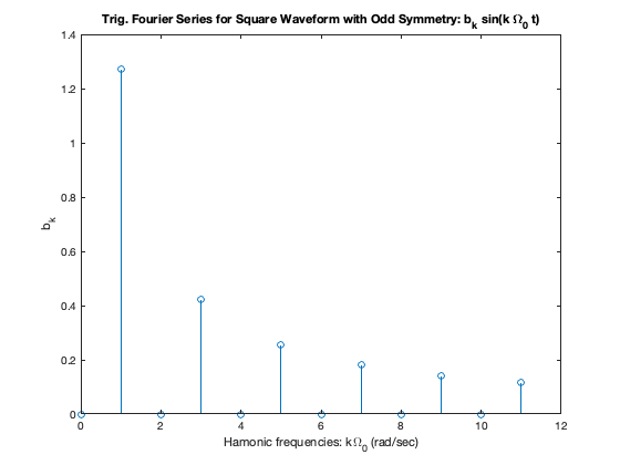
Fig. 3 Trigonometric Fourier series for a square wave#
Examples#
Example 3#
Compute the exponential Fourier series for the waveform shown below and plot its line spectra.
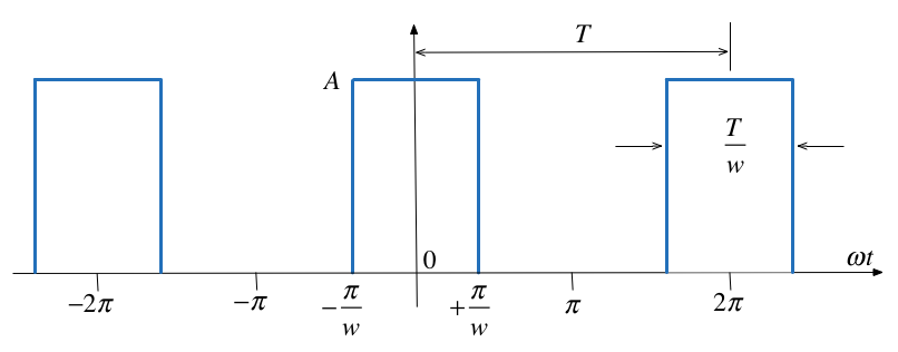
Fig. 4 A pulse train#
Solution#
The recurrent rectangular pulse is used extensively in digital communication systems. To determine how faithfully such pulses will be transmitted, it is necessary to know the frequency components.
What do we know?
The pulse duration is \(T/w\).
The recurrence interval \(T\) is \(w\) times the pulse duration.
\(w\) is the ratio of pulse repetition time to the pulse duration – normally called the duty cycle.
Coefficients of the Exponential Fourier Series?#
Given
Is the function even or odd?
Does the signal have half-wave symmetry?
What are the consequencies of symmetry on the form of the coefficients \(C_k\)?
What function do we actually need to integrate to compute \(C_k\)?
Practice here. Solutions at bottom of section.
DC Component?#
Let \(k = 0\) then perform the integral
Harmonic coefficients?#
Integrate for \(k\ne 0\)
Exponential Fourier Series?#
Example 4: Effect of pulse width on frequency spectra#
let’s see what effect the duty cycle \(w\) has on the spectra.
Recall pulse width = \(T/w\) and plot the complex line spectra for pulse with width \(w\) which repeats every \(T\) seconds. We will write a MATLAB function pulse_fs to simplify the computation.
clear all
cd ../matlab
format compact;
setappdata(0, "MKernel_plot_format", 'svg')
Copy the following text and save it in an m-file called pulse_fs.m
function [f,omega] = pulse_fs(A,w,range)
% PULSE_FS compute fourier series spectrum in range
% -range:range for pulse with
% height A, period T and width duty cycle w.
omega = -range:range;
for mm = 1:length(omega)
    x = omega(mm)*pi/w;
    if omega(mm) == 0
        f(mm) = A/w;
    else
        f(mm) = (A/w)*sin(x)/(x);
    end
end
return
edit pulse_fs
w = 2#
\(\Omega_0 = 1\) rad/s; \(w = 2\); \(T = 2\pi\) s; \(T/w = \pi\) s.
Compute Fourier series
A = 1; w = 2;
[f,omega] = pulse_fs(A,w,15);
Plot line Spectrum and add add continuous \(\mathrm{sinc}(x)\) envelope.
stem(omega,f)
title('Line Spectra for pulse with w=2')
hold on
om = linspace(-15,15,1000);
xlabel('k Omega_0 [rad/s]')
xc = om.*pi./w;

plot(om,(A/w)*sin(xc)./(xc),'r:')
hold off

w = 5#
\(\Omega_0 = 1\) rad/s; \(w = 5\); \(T = 2\pi\) s; \(T/w = \pi\) s.
A = 1; w = 5; [f,omega] = pulse_fs(A,w,15);
stem(omega,f)
title('Line Spectra for pulse with w=5')
hold on
om = linspace(-15,15,1000);
xlabel('k Omega_0 [rad/s]')
xc = om.*pi./w;
plot(om,(A/w)*sin(xc)./(xc),'r:')
hold off

w = 10#
\(\Omega_0 = 1\) rad/s; \(w = 10\); \(T = 2\pi\) s; \(T/w = \pi\) s.
A = 1; w = 10; [f,omega] = pulse_fs(A,w,15);
stem(omega,f)
title('Line Spectra for pulse with w=10')
hold on
om = linspace(-15,15,1000);
xlabel('k Omega_0 [rad/s]')
xc = om.*pi./w;
plot(om,(A/w)*sin(xc)./(xc),'r:')
hold off

Implications#
As the width of the pulse reduces the width of the freqency spectra needed to fully describe the signal increases
more bandwidth is needed to transmit the pulse.
Note
Text book seems to get the wrong results. Karris plots \(\sin(wx)/(wx)\) rather than \(\sin(x/w)/(x/w)\) in producing the diagrams shown in Figs. 7.36—7-38.
However, if you view \(\sin(wx)/wx\) as in indication of the bandwidth needed to transmit a pulse of width \(T/w\) the plots Karris gives make more sense.
Example 5#
Use the result of ex:18.1 to compute the exponential Fourier series of the impulse train \(\delta(t\pm 2\pi k)\) shown in {numref}`
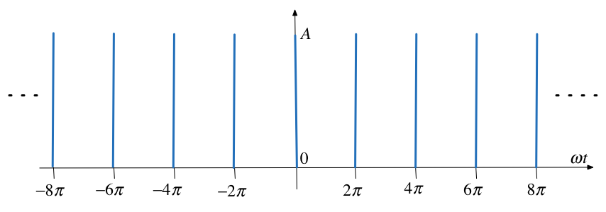
Fig. 5 An impulse train#
Solution#
To solve this we take the previous result and choose amplitude (height) \(A\) so that area of pulse is unity. Then we let width go to zero while maintaining the area of unity. This creates a train of impulses \(\delta(t\pm 2\pi k)\).
and, therefore
Try it!
Proof!#
From the previous result,
and the pulse width was defined as \(T/w\), that is
Let us take the previous impulse train as a recurrent pulse with amplitude
Pulse with unit area#
The area of each pulse is then
and the pulse train is as shown in Fig. 6 below:
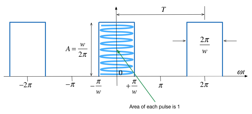
Fig. 6 Pulse train with unit-area pulses#
New coefficents#
The coefficients of the Exponential Fourier Series are now:
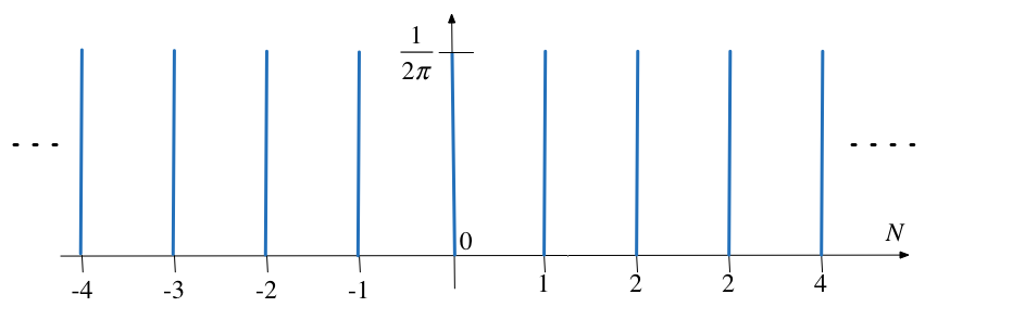
and as \(\pi/w \to 0\) each recurrent pulse becomes a unit impulse, and the pulse train reduces to a unit impulse train.
Also, recalling that
the coefficents reduce to
That is all coefficients have the same amplitude and thus
Spectrum of Unit Impulse Train#
The line spectrum of a sequence of unit impulses \(\delta(t \pm kT)\) is shown below:
Another Interesting Result#
Consider the pulse train again:
Fig. 7 Pulse train signal#
What happens when the pulses to the left and right of the centre pulse become less and less frequent? That is what happens when \(T \to \infty\)?
Well?#
As \(T\to \infty\) the fundamental frequency \(\Omega_0 \to 0\)
We are then left with just one pulse centred around \(t=0\).
The frequency difference between harmonics also becomes smaller.
Line spectrum becomes a continous function.
This result is the basis of the Fourier Transform which is coming soon.
Summary#
Unit 3.3: Takeways#
The exponential and trigonometric Fourier series coefficients can be plotted as lines on the frequency axis.
These line-spectra are useful for reasoning about the frequency components that are present in a periodic signal.
This is useful for e.g. computing the bandwidth needed on a medium that is to transmit a signal without loss.
We will see next, that we can also use these line spectra to compute power in a signal, the total harmonic distortion present in a signal, and in the design of filters.
Next Time#
We move on to consider
References#
Answer to example 3#
Given
Is the function even or odd? even \(f(t) = f(-t)\)!
Does the signal have half-wave symmetry? No!
What are the cosequencies of symmetry on the form of the coefficients \(C_k\)? \(C_k\) will be real values. Trig. equivalent no sine terms.
What function do we actually need to integrate to compute \(C_k\)? We only need to integrate between the limits \(-\pi/w \to \pi/w\)
Solution: DC component!#
or