6.2. Digital System Models and System Response
6.2.1. Digital System Models
The equivalent of the differential equation model for continuous systems is the difference equation for digital systems.
Replacing the differential operator \(\frac{d}{dt}\) by the advance operator \(\triangle\) gives the general form of the difference equation as
The equivalent of the differential equation model for continuous systems is the difference equation for digital systems.
6.2.1.1. Difference equation
Now, given the definition of the advance operator derived in a previous lecture
we can re-write equation (1) as the difference equation
6.2.1.2. Difference equation in terms of the delay operator
Unlike the differential equation, however, which is hardly ever expressed in an integral form, the difference equation is more usually expressed in terms of the delay operator \(\nabla\).
Applying the operator \(\nabla^n\) to equation (1) gives
### z-transform of difference equation
Applying the \(z\) transform directly to the difference equation with the delay operator (3) gives
6.2.1.3. z Transfer Function
Given that
The \(z\) transfer function is
A digital system in this general form is known as a “pole-zero, infinite impulse response, recursive auto-regressive moving average digital filter(!)”
6.2.1.4. z Transfer Function (2)
If \(b_1 = b_2 = \cdots = b_n = 0\) then the transfer function is
A digital system in this form is known as an “all pole, infinite impulse response, recursive auto-regressive digital filter.”
6.2.1.5. z Transfer Function (3)
When \(a_1 = a_2 = \cdots = a_n = 0\) then the transfer function is
A digital system in this form is known as an “all zero, finite impulse response, non recursive moving average digital filter.”
6.2.1.6. Other forms of digital transfer function
The transfer function can also be expressed in the zero-pole-gain form
and the partial fraction form
6.2.1.7. Canonical Forms
With the transfer function written as
there is a direct analogy with the general form of the continuous system transfer function with \(s\) instead of \(z\).
This was implemented with the physically realistic integral operator \(\int dt\) for which the digital equivalent is the delay operator \(\nabla\).
6.2.2. End of Pre-Class Presentation
This concludes the pre-class presentation.
In the class we will look at system response and compute the impulse and step responses of an example system.
6.2.3. Digital System Response
As in the case of a continuous system, the response of a digital signal comprises the sum of a free response and a forced response. The free response is dependent on the initial conditions of a digital system states, and as these are taken as zero here the free response is also zero and will not be considered further.
6.2.3.1. Digital System Response
The response of a digital system with transfer function \(H(z)\) to a digital input signal \(u\) is the digital output signal \(y\) given in transform form as
The inverse transform needed to determine the digital system response is obtained using the inverse z transform methods, e.g. polynomial division and partial fraction expansion, discussed in a previous lecture.
Taking the inverse transform gives the digital system response as
6.2.4. Response to Singularity Signals
The elemental singularity signals in a digital system response include the digital impulse signal and the digital step input.
6.2.4.1. Impulse response
6.2.4.1.1. Impulse signal
The digital impulse signal is given by
where \(\delta_0 = 1\) when \(k = 0\), and \(\delta_k = 0\) otherwise.
Therefore the sequence for the impulse is simply
The transform of the digital impulse signal is
6.2.4.1.2. Example 1: Impulse Response
Calculate the impulse response of the digital system with transfer function
Consider the system
The impulse response will be
We shall determine this response using the partial fraction expansion.
Assuming a partial fraction expansion of the form
we have
Gathering terms and equating coefficients
Hence
Thus
6.2.4.2. Step response
6.2.4.2.1. Step signal
The digital step signal is
where \(\epsilon_k = 1\) when \(k \ge 0\), and \(\epsilon_k = 0\) otherwise.
Therefore the sequence for the step is simply
6.2.4.2.2. z-transform of step signal
The transform of the digital step signal is
6.2.4.2.3. Example 2: Step Response
Calculate the step response of the digital system with transfer function
The step response of the example system is
We shall determine this response using the partial fraction expansion.
Earlier we showed that the result of the partial fraction expansion was
and the corresponding sequence is
6.2.5. Computing Digital System Responses with MATLAB
We will run this part of the presentation in class. There is an executable version as a MATLAB Live Script available as digiresp.mlx.
6.2.5.1. Control System Toolbox Help
What functions do we have in the controls system toolbox?
imatlab_export_fig('print-svg') % Static svg figures.
doc control
6.2.5.1.2. Transfer function
From this, the transfer function looks likely
help tf
 TF  Construct transfer function or convert to transfer function.

   Construction:
     SYS = TF(NUM,DEN) creates a continuous-time transfer function SYS with
     numerator NUM and denominator DEN. SYS is an object of type TF when
     NUM,DEN are numeric arrays, of type GENSS when NUM,DEN depend on tunable
     parameters (see REALP and GENMAT), and of type USS when NUM,DEN are
     uncertain (requires Robust Control Toolbox).

     SYS = TF(NUM,DEN,TS) creates a discrete-time transfer function with
     sample time TS (set TS=-1 if the sample time is undetermined).

     S = TF('s') specifies the transfer function H(s) = s (Laplace variable).
     Z = TF('z',TS) specifies H(z) = z with sample time TS.
     You can then specify transfer functions directly as expressions in S
     or Z, for example,
        s = tf('s');  H = exp(-s)*(s+1)/(s^2+3*s+1)

     SYS = TF creates an empty TF object.
     SYS = TF(M) specifies a static gain matrix M.

     You can set additional model properties by using name/value pairs.
     For example,
        sys = tf(1,[1 2 5],0.1,'Variable','q','IODelay',3)
     also sets the variable and transport delay. Type "properties(tf)"
     for a complete list of model properties, and type
        help tf.<PropertyName>
     for help on a particular property. For example, "help tf.Variable"
     provides information about the "Variable" property.

     By default, transfer functions are displayed as functions of 's' or 'z'.
     Alternatively, you can use the variable 'p' in continuous time and the
     variables 'z^-1', 'q', or 'q^-1' in discrete time by modifying the
     "Variable" property.

   Data format:
     For SISO models, NUM and DEN are row vectors listing the numerator
     and denominator coefficients in descending powers of s,p,z,q or in
     ascending powers of z^-1 (DSP convention). For example,
        sys = tf([1 2],[1 0 10])
     specifies the transfer function (s+2)/(s^2+10) while
        sys = tf([1 2],[1 5 10],0.1,'Variable','z^-1')
     specifies (1 + 2 z^-1)/(1 + 5 z^-1 + 10 z^-2).

     For MIMO models with NY outputs and NU inputs, NUM and DEN are
     NY-by-NU cell arrays of row vectors where NUM{i,j} and DEN{i,j}
     specify the transfer function from input j to output i. For example,
        H = tf( {-5 ; [1 -5 6]} , {[1 -1] ; [1 1 0]})
     specifies the two-output, one-input transfer function
        [     -5 /(s-1)      ]
        [ (s^2-5s+6)/(s^2+s) ]

   Arrays of transfer functions:
     You can create arrays of transfer functions by using ND cell arrays
     for NUM and DEN above. For example, if NUM and DEN are cell arrays
     of size [NY NU 3 4], then
        SYS = TF(NUM,DEN)
     creates the 3-by-4 array of transfer functions
        SYS(:,:,k,m) = TF(NUM(:,:,k,m),DEN(:,:,k,m)),  k=1:3,  m=1:4.
     Each of these transfer functions has NY outputs and NU inputs.

     To pre-allocate an array of zero transfer functions with NY outputs
     and NU inputs, use the syntax
        SYS = TF(ZEROS([NY NU k1 k2...])) .

   Conversion:
     SYS = TF(SYS) converts any dynamic system SYS to the transfer function
     representation. The resulting SYS is always of class TF.

   See also TF/EXP, FILT, TFDATA, ZPK, SS, FRD, GENSS, USS, DYNAMICSYSTEM.

    Documentation for tf
       doc tf

    Other functions named tf

       DynamicSystem/tf    idParametric/tf    mpc/tf    StaticModel/tf
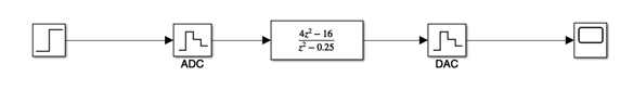
6.2.5.1.3. Digital transfer function block
It seems that that the third argument is sampling period. Set this to -1 for “unspecified”.
H = tf([4, 0, -16],[1, 0, -0.25],-1)
H =
4 z^2 - 16
----------
z^2 - 0.25
Sample time: unspecified
Discrete-time transfer function.
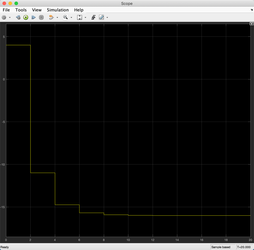
6.2.5.2. Step Response
Now do a step response
step(H)

What about the sequence values?
ys = step(H)
ys =
    4.0000
    4.0000
  -11.0000
  -11.0000
  -14.7500
  -14.7500
  -15.6875
  -15.6875
  -15.9219
  -15.9219
  -15.9805
  -15.9805
  -15.9951
  -15.9951
  -15.9988
  -15.9988
  -15.9997
  -15.9997
  -15.9999
  -15.9999
  -16.0000
Does the sequence match the theory?
6.2.5.3. Impulse Response
How about impulse response?
impulse(H)

The plot isn’t quite right – it’s a “hold-equivalent” result. We don’t know values between sampling instants.
Sequence?
yi = impulse(H)
yi =
    4.0000
         0
  -15.0000
         0
   -3.7500
         0
   -0.9375
         0
   -0.2344
         0
   -0.0586
         0
   -0.0146
         0
   -0.0037
         0
   -0.0009
         0
   -0.0002
         0
   -0.0001


6.2.5.4. Partial fractions
Can we use partial fractions for inverse z transforms?
help residue
 RESIDUE Partial-fraction expansion (residues).
    [R,P,K] = RESIDUE(B,A) finds the residues, poles and direct term of
    a partial fraction expansion of the ratio of two polynomials B(s)/A(s).
    If there are no multiple roots,
       B(s)       R(1)       R(2)             R(n)
       ----  =  -------- + -------- + ... + -------- + K(s)
       A(s)     s - P(1)   s - P(2)         s - P(n)
    Vectors B and A specify the coefficients of the numerator and
    denominator polynomials in descending powers of s.  The residues
    are returned in the column vector R, the pole locations in column
    vector P, and the direct terms in row vector K.  The number of
    poles is n = length(A)-1 = length(R) = length(P). The direct term
    coefficient vector is empty if length(B) < length(A), otherwise
    length(K) = length(B)-length(A)+1.

    If P(j) = ... = P(j+m-1) is a pole of multplicity m, then the
    expansion includes terms of the form
                 R(j)        R(j+1)                R(j+m-1)
               -------- + ------------   + ... + ------------
               s - P(j)   (s - P(j))^2           (s - P(j))^m

    [B,A] = RESIDUE(R,P,K), with 3 input arguments and 2 output arguments,
    converts the partial fraction expansion back to the polynomials with
    coefficients in B and A.

    Warning: Numerically, the partial fraction expansion of a ratio of
    polynomials represents an ill-posed problem.  If the denominator
    polynomial, A(s), is near a polynomial with multiple roots, then
    small changes in the data, including roundoff errors, can make
    arbitrarily large changes in the resulting poles and residues.
    Problem formulations making use of state-space or zero-pole
    representations are preferable.

    Class support for inputs B,A,R:
       float: double, single

    See also POLY, ROOTS, DECONV.

    Documentation for residue
       doc residue
6.2.5.4.1. PFE for for inverse z-transform of impulse response
[r,p,k] = residue([4,0,-16],[1,0,-0.25])
r =
   -15
    15
p =
    0.5000
   -0.5000
k =
     4
6.2.5.4.2. PFE for inverse z-transform for step response
[r,p,k] = residue(conv([1, 0],[4,0,-16]),conv([1, -1],[1,0,-0.25]))
r =
  -16.0000
   15.0000
    5.0000
p =
    1.0000
    0.5000
   -0.5000
k =
     4
Do these results match the theory?
6.2.5.4.3. Another approach
Use LTI block to define the TF then extract num/den for PFE
U = tf([1, 0], [1, -1], -1)
Y = series(U, H)
U =
z
-----
z - 1
Sample time: unspecified
Discrete-time transfer function.
Y =
4 z^3 - 16 z
-------------------------
z^3 - z^2 - 0.25 z + 0.25
Sample time: unspecified
Discrete-time transfer function.
extract numerator & denominator
[num,den] = tfdata(Y,'v')
num =
     4     0   -16     0
den =
    1.0000   -1.0000   -0.2500    0.2500
get pfe
[r,p,k]=residue(num,den)
r =
  -16.0000
   15.0000
    5.0000
p =
    1.0000
    0.5000
   -0.5000
k =
     4