3.4. Cascade Lead compensation¶

3.4.1. Introduction¶

The proportional plus derivative compensator has the unfortunate property that its high frequency gain is infinite. This means that high frequency effects, such as sensor noise and un-modelled high-frequency dynamics, e.g. resonance terms, will be amplified with potentially disastrous effects. Of course, a real physical derivative operator cannot be implemented and any implementation will actually have poles that will limit the high-frequency gain.

Recognizing this, an alternative to the pure P+D

$D_{\mathrm{P+D}}=K_D s + K_{\mathrm{prop}}$

is the so-called “lead compensator”

$D_{\rm{lead}}(s) = {K_c}\left( \frac{s - z_0}{s - p_0}\right)$

where

$|p_0| > |z_0|.$

Considering the frequency response of $D_{\mathrm{lead}}$

$D_{\mathrm{lead}}(j\omega) = K_c\left(\frac{j\omega-z_0}{j\omega-p_0}\right)$

The low and high-frequency gains are:

$\left.D_{\mathrm{lead}}(j\omega)\right|_{\omega\to 0} = Kc \left(\frac{z_0}{p_0}\right)$

$\left.D_{\mathrm{lead}}(j\omega)\right|_{\omega\to \infty} = Kc$

so that the ratio of high-to-low frequency gain is

$\frac{D_{\mathrm{lead}}(j\infty)}{D_{\mathrm{lead}}(j0)}=\frac{p_0}{z_0}>0$

The lead compensator is still a high-pass filter but the pole at $s=p_0$ limits the high frequency gain. Typically, the ratio of $p_0$ to $z_0$ is kept to below 10.

3.4.2. Properties of the Cascade Lead Compensator¶

As $|p_0| > |z_0|$ , the angle contributed by the compensator to some arbitrary point $s_1$ at on the s-plane is illustrated in Figure 1.

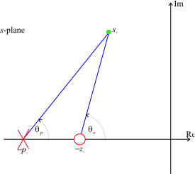
Figure 1 Angle contribution of a lead compensator

The net contribution is

$\phi_c = \theta_z - \theta_p > 0$

so that the lead compensator always makes a positive contribution to the angle criterion.

This has the effect of allowing the closed-loop poles to move to the left in the s-plane.

The problem is then how to choose the relative location of the pole and the zero.

We reproduce the advice of D’Azzo and Houpis (1975).

3.4.3. Method 1¶

Use the zero to cancel a low frequency real pole. This can simplify the root locus and reduce the complexity of the problem. The compensator pole is then placed such that $s_1$ becomes a point on the desired root-locus.

For a Type 1 system, the real pole (excluding the pole at zero) that is closest to the origin should be cancelled.

For a Type 0 system, the second closest pole to the origin should be cancelled.

3.4.3.1. Example 1¶

The following Matlab code illustrates these principles for the system with

Type 1 open-loop transfer function

$G_1(s) = \frac{1}{s(s + 1)}$

Define the plant

G1 = tf(1,conv([1, 0],[1, 1])); H=1;

Plot root-locus

rlocus(G1*H)

Clearly, we cannot achieve a closed-loop pole at $s_1 = -2 + j2$ without some dynamic compensation.

However, if we use the zero of a cascade lead compensator to cancel the pole at $s = -1$ and place the pole at $s = -4$ we get:

D1 = zpk([-1],[-4],1);
Go1 = D1*G1*H;

rlocus(Go1)

which will have a closed-loop pole at the desired location when the gain is

Kc = rlocfind(Go1,-2+2j)

Kc =
     8

3.4.3.2. Example 2¶

For a Type 0 system

$G_2(s) = \frac{1}{(s + 1)(s + 2)}$

the zero should be used to cancel the pole at $s=-2$ . We leave it as an exercise to prove that the compensator

$D_2(s)=5\left(\frac{s+2}{s+3}\right)$

gives the desired closed-loop poles.

Note

You should be aware that the lead compensator zero will still appear in the closed-loop transfer function, and you should verify that the closed-loop step response is acceptible.

3.4.4. Method 2¶

The following graphical method maximizes the ratio between pole and zero for any given angle contribution. This minimizes the additional compensator gain needed to satisfy the gain criterion.

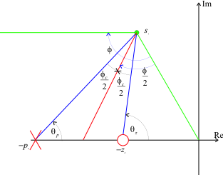Figure 2 Graphical construction for locating the pole and zero of a lead compensator.

The steps in the location of the lead-compensator pole and zero are as follows (refer to Figure 2).

Locate the desired closed-loop pole $s_1$ . Draw a line from the origin to $s_1$ and a horizontal line through $s_1$ to the left.

Bisect the angle between the two lines drawn in step 1.

Measure the angle $\phi_c$ either side of the line drawn in step 2.

The intersections of these lines with the real axis locate the compensator pole $p_0$ and zero $z_0$ .

3.4.4.1. Example 3¶

We return to the satellite attitude control problem with

$G(s) = \frac{1}{s^2}$

Requiring a closed-loop pole $S_1 = -2 + j2$ , the geometry of the problem is illustrated in Figure 3.

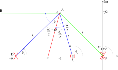Figure 3 Lead compensator design for the satellite attitude control problem.

Note that the line drawn from the origin to the point s1 subtends an angle of $135^\circ$ to the positive real axis.

We can use MATLAB to help to work through the trigonometry. The angle contribution of the plant and feedback at $s_1$ is obtained as follows.

G = tf(1,[1,0,0]);
H = 1;
GH = G*H;
s1 = -2+2j;

The total contribution of the plant poles and zeros can be calculated directly using the Matlab equivalent of the angle criterion

[zeros,poles,gain]=zpkdata(GH,'v');

contribution in degrees

contrib = (180/pi)*(sum(angle(s1 - zeros)) - sum(angle(s1 - poles)))

contrib =
  -270

The root locus angle criterion gives lead contribution

$\begin{split}\begin{array}{c}\angle G({s_1})H({s_1}) + {\phi _c} = - {180^ \circ }\\{\phi _c} = - {180^ \circ } - \angle G({s_1})H({s_1})\end{array}\end{split}$

phi_c = -180 - contrib

phi_c =
    90

half_phi_c = phi_c/2

half_phi_c =
    45

Because the line BA and OD are parallel, the angle subtended by the line OAB is also $135^\circ$ . Thus

angle_OAB = 135;
angle_BAD = angle_OAB/2 - half_phi_c;
angle_BEO = angle_OAB/2 + half_phi_c;

and by parallel line theory

theta_p = angle_BAD

theta_p =
   22.5000

theta_z = angle_BEO

theta_z =
  112.5000

The pole and zero locations are given by

p0 = -2-2/tan(theta_p*pi/180)

p0 =
   -6.8284

z0 = -2-2/tan(theta_z*pi/180)

z0 =
   -1.1716

The compensator gain is obtained using the gain criterion. With MATLAB, this can be calculated directly from the gain formula:

${K_0} = \left( \frac{\left| s_1 - p_0 \right|}{\left| s - z_0 \right|} \right)\left( \frac{\prod\limits_{i = 1}^{n - 1} \left| s_1 - p_i \right| }{\prod\limits_{j = 1}^{n - 1} \left| s_1 - z_j \right|} \right)$

Ko = (abs(s1-p0)*prod(abs(s1-poles)))/(abs(s1-z0)*prod(abs(s1-zeros)))

Ko =
   19.3137

Let us also check this result using the root locus.

D = zpk(z0,p0,1);
Go=D*GH;
rlocus(Go)

Kc = rlocfind(Go,s1)

Kc =
   19.3137

Finally, let us calculate the step response and compare it with the result achieved with velocity feedback

$G_1(s) = \frac{8}{s^2 + 4s + 8}$

and proportional + derivative compensation

$G_2(s) = \frac{4(s+2)}{s^2 + 4s + 8}$

G1 = tf(8,[1, 4, 8]);
G2 = tf(4*[1, 2],[1, 4, 8]);
G3 = feedback(Kc*D*G,H)

G3 =

      19.314 (s+1.172)

  ------------------------

  (s+2.828) (s^2 + 4s + 8)

Continuous-time zero/pole/gain model.

[y1,t1]=step(G1);
[y2,t2]=step(G2);
[y3,t3]=step(G3);
plot(t1,y1,t2,y2,t3,y3),legend('Velocity fb','P+D','cascade lead'),title('Lead compensation: Comparison of results')

When evaluating the third design you should take into account the location of the compensator zero and the third closed-loop pole (at $s = -2.828$ ) relative to the desired closed-loop pole at $s_1$ .

3.4.5. Method 3¶

The third method referenced in D’Azzo and Houpis addresses a problem with lead compensator design that has so far not been addressed. That is that only the desired transient performance, and hence the desired location of the dominant closed-loop poles, is considered. The desired system gain is not specified. A method of achieving both gain and desired pole location has been proposed by Phillips and Harbour (1988) and is considered in the Analytic Root Locus Design section (not assessed).

3.4.6. References¶

John J. D’Azzo and Constantne Houpis, (1975) Linear Control System Analysis and Design (Conventional and Modern), McGraw & Hill, 1975 and later editions.

Phillips and Harbor (1988), Feedback Control Systems, Prentice Hall.

3.4.7. Resources¶

An executable version of this document is available to download as a MATLAB Live Script file cclead.mlx.

The Simulink model which compares the results of the satellite attitude control system compensated with velocity feedback, P+D compensation and lead compensation is lead_compensation.slx.

EGLM03 Modern Control Systems