3.3. Proportional Plus Derivative Compensation¶

3.3.1. Introduction¶

First design example (Satellite Attitude Control).

Plant: $ $G(s) = \frac{1}{s^2}$ $

Feedback:

$H(s) = 1$

With velocity feedback the system is as shown in Figure 1.

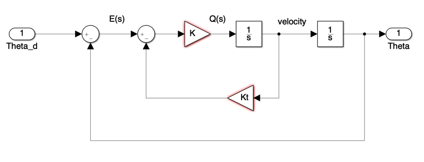Figure 1 Satellite Attitude Control with Velocity Feedback

For this system, the root locus equation is

$1+\frac{KK_T \left(s+\frac{1}{K_T }\right)}{s^2 }$

and the design parameters where calculated to be

Kt = 0.5; K = 8;

The closed-loop characteristic equation is

clce1 = [1, K*Kt, K];

The closed-loop transfer function is then:

Gc1 = tf(K,clce1)

Gc1 =

  -------------

  s^2 + 4 s + 8

Continuous-time transfer function.

In this document we illustrate how we may implement a silimilar control law using cascade compensation.

3.3.2. Cascade compensator¶

An alternative compensation architecture is the cascade compensator illustrated in Figure 2.

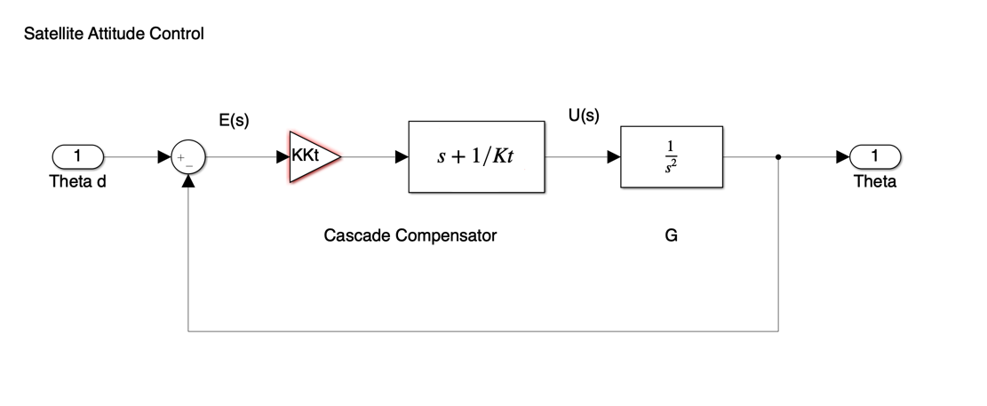Figure 2 The cascade compensator

The compensator is in series with the plant so that, in general, if the compensator transfer function is

$D(s)=\frac{K_c(s+z_1)\ldots(s+z_r)}{(s+p_1)\ldots(s+p_q)}$

and the compensator poles and zeros are simply added to the poles and zeros of the plant.

If we wish to achieve the same root-locus equation as the previous design (1) then the compensator must have transfer function

$D(s) = K_c(s + z_1)$

where

$K_c = K K_t = 4$

$z_1 = 1/K_t = 2$

Let us verify that this gives the same results as the previous example:

Kt = 1/2;
z1 = -1/Kt;
Go = zpk(z1,[0, 0],1) % root locus gain initially set to unity

Go =

  (s+2)

  -----

s^2

Continuous-time zero/pole/gain model.

rlocus(Go),title('Root locus for cascade compensated system')

Find the root locus gain at the point on the root locus where the poles are located at $s=-2+j2$ .

Kc = rlocfind(Go,-2+2j)

Kc =
     4

Now add this to the compensator

D = tf(Kc*[1 -z1],1)

D =

  4 s + 8

Continuous-time transfer function.

$D(s) = 4s + 8$

Analysis of this compensator reveals that it is of a type known as “proportional plus derivative” (P+D). The output of the compensator is of the form

$U(s) = K_DsE(s)+K_{\mathrm{prop}}E(s)$

$u(t) = K_d\frac{de(t)}{dt}+K_{\mathrm{prop}}e(t)$

and is made up of a “proportion” of the error plus a proportion of the rate-of-change (or derivative) of the error. It is the derivative term that gives the dampening effect required to allow the frictionless system to come to rest.

3.3.3. Closed-loop response¶

The closed-loop tranfer function is given by

$G_c(s) = \frac{D(s)G(s)}{1+D(s)G(s)}$

G=tf(1,[1,0,0])

G =

---

s^2

Continuous-time transfer function.

Gc2 = feedback(D*G,1)

Gc2 =

     4 s + 8

  -------------

  s^2 + 4 s + 8

Continuous-time transfer function.

Let us plot and compare the step responses of the P+D and velocity feedback results.

[y1,t1]=step(Gc1);
[y2,t2]=step(Gc2);
plot(t1,y1,t2,y2),...
 legend('Velocity fb','P+D'),...
 title('Step response: closed-loop compensated system')

      
    

3.3.4. Notes¶

Notice that, although the settling time is about the same in both designs, the overshoot is considerably larger in the P+D compensated system. This is because the zero added by the P+D compensator appears in the numerator of the closed-loop transfer function. (refer back to Contact Hour 2 for an explanation).

3.3.5. Resources¶

An executable version of this document is available to download as a MATLAB Live Script file pplusd.mlx.

The Simulink model of the satellite attitude control system with P+D compensation is satellite.slx.

EGLM03 Modern Control Systems