3.2. Introduction to Root Locus Design¶

In this section we will engage in a short exploration of compensator design in the time domain with a look at root-locus design of a velocity-feedback compensator for a simple “double integrator” system. This serves as an introduction to the topic of phase lead compensation which is used to improve transient performance and relative stability.

3.2.1. Gain compensation¶

First design example (Satellite Attitude Control). The system may be represented in block diagram form as shown in Figure 1. (Simulink model: satellite.slx)

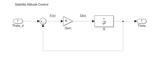
Satellite control with gain modulated torque

Figure 1 Satellite control with gain modulated torque

For this system the plant transfer function is

\[G(s) = \frac{1}{s^2}\]

Feedback:

\[H(s) = 1\]

Controller:

\[D(s) = K\]

The root locus equation is:

\[1 + KG(s)H(s) = 0\]

with root locus parameter = \(K\).

Defining the problem in Matlab

G = tf(1,conv([1,0],[1,0]));
H = tf(1,1);
Go = G*H

Go =

---

s^2

Continuous-time transfer function.

Note: The root locus gain \(K\) is implied in Matlab (it does not need to be defined)

rlocus(Go),title('Root locus diagram for gain modulated satellite attitude control')

Pick off an arbitrary gain

[K]=rlocfind(Go,3/4j)

K =
    0.5625

Closed-loop transfer function

Gc = feedback(K*G,H)

Gc =

     0.5625

  ------------

  s^2 + 0.5625

Continuous-time transfer function.

\[G_c(s) = \frac{0.5625}{s^s + 0.5625}\]

step(Gc,45),title('Step response for closed-loop system with K=sqrt(3)/2')

3.2.2. With velocity feedback,¶

The block diagram becomes that shown in Figure 2 (Simulink model: velfb.slx).

velfb

The root locus equation is

\[1 + \frac{KK_T(s + 1/K_T)}{s^2} = 0\]

where \(KK_T\) is the root locus gain.

System with velocity feedback

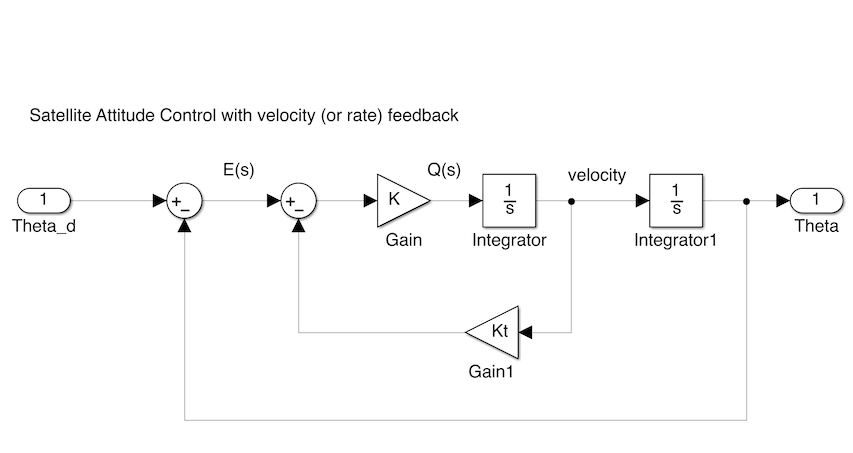
Figure 2 System with velocity feedback

Kt = 0.5;
Go2=tf(Kt*[1, 1/Kt],[1,0,0]);
rlocus(Go2),title('Root locus of system with velocity feedback')

3.2.3. Closed-loop step response¶

\[G_o(s)=\frac{1}{s}\times \frac{K/s}{1 + (KK_T)/s}\]

\[G_o(s)= \frac{K}{s(s + KK_T)}\]

\[G_c(s) = \frac{K}{s^2 + KK_T s + K}\]

[K] = rlocfind(Go2,-2+2j)

K =
     8

Integrator=tf(1,[1,0]);
G1=feedback(K*Integrator,Kt)*Integrator;
Gc2=feedback(G1,1)

Gc2 =

  -------------

  s^2 + 4 s + 8

Continuous-time transfer function.

step(Gc2),title('Step response for velocity feedback (rate) compensated system')

Since \(KK_t = 4\)

Kt = 4/K

Kt =
    0.5000

Running the simulink model with these values should give you the same result.

3.2.4. Resources¶

An executable version of this document is available to download as a MATLAB Live Script file velfb.mlx.

The Simulink model of the satellite attitude control system is satellite.slx.

The system with velocity feedback control is available as velfb.slx.

EGLM03 Modern Control Systems

3.2. Introduction to Root Locus Design¶

3.2.1. Gain compensation¶

3.2.2. With velocity feedback,¶

3.2.3. Closed-loop step response¶

3.2.4. Resources¶